Exploring R package contributor data on GitHub with the {tidyverse}, {gh}, and {tidygraph}.
.Wrangle
.Visualize
{tidyverse}
{gh}
{gt}
{ggrepel}
{scales}
{igraph}
{tidygraph}
{ggraph}
{graphlayouts}
Author
Michael McCarthy
Published
May 10, 2023
Overview
In my previous post I explored R package developer statistics on CRAN, focusing on developers with package authorship. However, because many of the packages published on CRAN are hosted on open source repositories (like GitHub), many R packages have additional contributors who do not appear in the list of authors.
@mccarthymg Very interesting (though not surprising)!
One caveat is that most big packages have many more contributors than declared authors, because people often only submit a handful of patches, and are consequently not added you the authors list (to be clear, I don't think that's a problem; just something to keep in mind).
Although this information isn’t available through CRAN, GitHub has a REST API that we can use to get data on the contributors of R packages hosted on GitHub. We can use this to answer new questions about R package contributions by the wider R community.
Again, if you just want to see the stats, you can skip to the R contributor statistics section. Otherwise follow along to see how I retrieved and wrangled the data into a usable state. I’d also like to give a big thanks to everyone who engaged with me on my previous post (and some of the stuff in-between); you all inspired this post and some of the approaches I chose to take below.
I’ll be using the CRAN package repository data returned by tools::CRAN_package_db() again in this post, this time to get the following DESCRIPTION fields from each package: BugReports and URL. Each of these fields can contain the URL for a package’s GitHub repository, so I’m taking both for better coverage.
Since this data will change over time, here’s when tools::CRAN_package_db() was run for reference: 2023-05-06.
I’ve also selected the Author and Authors@R fields again so I can rerun the author extraction code from the previous post. This will let us ask more interesting questions later on. I just need package and author names, so the code is slightly different from the previous post.
I’ve hidden the code since there’s no need to reexplain it—all that matters is that this returns a two column data frame called cran_authors, with columns package and person.
Code
# Helper functions ------------------------------------------------------------# Get names from "person" objects in the Authors@R fieldauthors_r <-function(x) { code <-str_replace_all(x, "\\<U\\+000a\\>", "\n") persons <-eval(parse(text = code)) person <-str_trim(format(persons, include =c("given", "family")))tibble(person = person)}# Get names from character strings in the Author fieldpersons_roles <- r"((\'|\")*[A-Z]([A-Z]+|(\'[A-Z])?[a-z]+|\.)(?:(\s+|\-)[A-Z]([a-z]+|\.?))*(?:(\'?\s+|\-)[a-z][a-z\-]+){0,2}(\s+|\-)[A-Z](\'?[A-Za-z]+(\'[A-Za-z]+)?|\.)(?:(\s+|\-)[A-Za-z]([a-z]+|\.))*(\'|\")*(?:\s*\[(.*?)\])?)"person_objects <- r"(person\((.*?)\))"authors <-function(x) { persons <- x |>str_replace_all("\\n|\\<U\\+000a\\>|\\n(?=[:upper:])", " ") |>str_replace_all("\\.", "\\. ") |>str_remove_all(",(?= \\[)") |>str_extract_all(paste0(persons_roles, "|", person_objects)) |>unlist() |>str_replace_all("\\s+", " ")tibble(person = persons) |>mutate(person =str_remove(str_remove(person, "\\s*\\[(.*?)\\]"),"^('|\")|('|\")$" ) )}# Get data used in the previous post ------------------------------------------cran_authors <- cran_pkgs_db |>select(package, authors, authors_r) |>as_tibble() |>mutate(across(c(authors, authors_r), \(.x) stri_trans_general(.x, "latin-ascii")),persons =if_else(is.na(authors_r),map(authors, \(.x) authors(.x)),map(authors_r, \(.x) authors_r(.x)) ) ) |>select(-c(authors, authors_r)) |>unnest(persons) |># Some unicode characters from authors_r were sneaking through despite the# first normalization call. Also making everything title case to improve# joining results later.mutate(person =str_to_title(stri_trans_general(person, "latin-ascii")))
Wrangle
I’ll be using the gh package to query GitHub’s REST API. However, before any queries can be done, I need to figure out which packages in cran_pkgs_db have GitHub repositories and what their URLs are.
Finding the packages with GitHub repositories is simple—it’s just a matter of filtering cran_pkgs_db down to the subset of packages with GitHub’s base URL.
Of the 19483 packages on CRAN, 9182 have a GitHub URL in the BugReports or URL field.
Next step: get the repository URLs. Again, regular expressions are our friend. This one is a simple search for the owner and repository name following the GitHub base URL in the form of owner/repo, following GitHub’s rules for the allowable characters in user and repository names. After getting that it’s just a matter of tidying the data up a bit more to make it query-ready.
owner_repo <- r"((?<=https:\/\/github.com\/)([A-Za-z0-9\-]{1,39}\/[A-Za-z0-9\-\_\.]+))"cran_gh_repos <- cran_gh_repos |>mutate(# Get the owner and repo name from a GitHub URL in the form: owner/repoacross(c(bug_reports, url), \(.x) str_extract(.x, owner_repo)),repo_url =case_when(# There shouldn't be a need to check for both columns being NA, since# at least one column should have the info we want due to the filter()# call at the start of this pipe.is.na(bug_reports) &!is.na(url) ~ url,!is.na(bug_reports) &is.na(url) ~ bug_reports, bug_reports == url ~ bug_reports ),# We just need everything before or after the / to get the owner and repo.owner =str_extract(repo_url, ".+(?=\\/)"),repo =str_extract(repo_url, "(?<=\\/).+") ) |>select(package, owner, repo) |># Despite the previous comment, some packages only include their username# or organization in the URL, which we can't make use of and which return# NA. These should be omitted. There aren't that many (< 100).na.omit()cran_gh_repos
The GitHub REST API has a rate limit of 5000 requests per hour for authenticated users, so the repositories have to be queried in chunks instead of doing them all in one go. To accomodate this, cran_gh_repos can be split into a list of data frames that can be mapped over when calling the API. I’ve chosen groups of 4000 here just to avoid accidentally hitting the limit.
n_per_group <-4000n_groups <-ceiling(nrow(cran_gh_repos)/n_per_group)query_groups <- cran_gh_repos |>mutate(# The result of the rep() call needs to be subset to the max number of# observations to avoid a recycling error with vctrs.query_group =paste0("group_", rep(1:n_groups, each = n_per_group)[1:nrow(cran_gh_repos)] ) ) |>group_by(query_group) |>nest() |>deframe()query_groups
We’re now ready to get the contributors for each package. The code here is based on the code used to thank contributors in the R for Data Science book, so if you want to understand the general idea I’d recommend running that code. Otherwise this is just an extension of that code, using list columns, rectangling, and error handling to make it work over multiple repositories.
contributors_all <- query_groups |>map_dfr( \(query_group) {# All packages will be queried within the group one-by-one. We just# need package names, usernames, and commit numbers; everything else# can be dropped. query_result <- query_group |>rowwise() |>mutate(contributors_json =list(# Some package repos don't exist anymore (404), which triggers an# error. This needs to be handled in order for the rest of the# queries to continue running.tryCatch(expr = { gh::gh("/repos/:owner/:repo/contributors",owner = owner,repo = repo,.limit =Inf ) },error = \(unused_argument) {# For consistency with `gh()`, return a list with the keys we# want but with NA values.list(list(login =NA_character_, contributions =NA_integer_)) } ) ),contributors =list(tibble(login =map_chr(contributors_json, "login"),n_commits =map_int(contributors_json, "contributions") )) ) |>select(-c(owner, repo, contributors_json)) |>unnest(contributors)# Once a group is done, rest for an hour to avoid the rate limit.Sys.sleep(3600) query_result } )contributors_all
As you can see from the output above, contributors are returned as logins rather than names; so the API will need to be queried a second time to get the names corresponding to each login. However, to avoid redundancy and reduce the total number of queries, we should only take the unique login names from the contributor data.
# We only want real people, not bots or other automated tools. Most bots have a# common naming scheme for their login, but there are exceptions. May as well# drop the NA entries here too, since it's convenient.contributors_all <- contributors_all |>filter(!( login %in%c("actions-user","cran-robot","fossabot","ImgBotApp","traviscibot",NA_character_ ) |str_detect(login, "\\[bot\\]$|\\-bot$") ) )contributors_unique <-tibble(login =unique(contributors_all$login))contributors_unique
We also need to make query groups for contributors_unique to avoid hitting the rate limit, since logins need to be queried one-by-one.
# We need to make query groups here too to avoid hitting the rate limit.n_per_group <-4000n_groups <-ceiling(nrow(contributors_unique)/n_per_group)query_groups <- contributors_unique |>mutate(query_group =paste0("group_", rep(1:n_groups, each = n_per_group)[1:nrow(contributors_unique)] ) ) |>group_by(query_group) |>nest() |>deframe()query_groups
Again, this query is just a generalization of the R for Data Science contributors code. Here we’re getting users’ real names from their login names, then tidying up.
contributors_tidy <- query_groups |>map_dfr( \(query_group) {# All logins will be queried within the group one-by-one. query_result <- query_group |>rowwise() |>mutate(users_json =list(# Some user login names don't exist anymore (404), which triggers# an error. This needs to be handled in order for the rest of the# queries to continue running.tryCatch(expr = { gh::gh("/users/:username", username = login) },error = \(unused_argument) {# For consistency with `gh()`, return a list with the keys we# want but with NA values.list(list(login = login, name =NA_character_)) } ) ),# Some users don't have a name filled out. To keep it from being# empty, use their login name instead.name =pluck(users_json, "name", .default = login) ) |># Rowwise evaluation is no longer needed and I don't want active after# this code chunk.ungroup() |># Letters with accents, etc. should be normalized so that they match# the normalized names in `cran_authors` from the previous post.mutate(name =str_trim(stri_trans_general(name, "latin-ascii"))) |>select(name, login)# Once a group is done, rest for an hour to avoid the rate limit.# Since this is our last query, there's a redundant hour of waiting# after the last query group is finished. This is easy to fix, but I'm# only running this code once *ever*, so it's even easier not to.Sys.sleep(3600) query_result } )contributors_tidy
#> # A tibble: 15,318 × 2
#>    name           login
#>    <chr>          <chr>
#>  1 Spiritspeak    Spiritspeak
#>  2 Sigbert Klinke sigbertklinke
#>  3 Wenjie Wang    wenjie2wang
#>  4 Dennis Prangle dennisprangle
#>  5 Kyle Bittinger kylebittinger
#>  6 Jin Zhu        Mamba413
#>  7 Junhao Huang   oooo26
#>  8 Jiang-Kangkang Jiang-Kangkang
#>  9 Liyuan Hu      zaza0209
#> 10 bbayukari      bbayukari
#> # … with 15,308 more rows
Tidying GitHub query results
With the names associated with each login in contributors_tidy, I can add those to contributors_all.
contributors_all <- contributors_all |>left_join(contributors_tidy) |>relocate(name, .before = login) |># Make all names title case to improve the success rates of joining names# with `cran_authors` in the next code chunk.mutate(name =str_to_title(name))contributors_all
Even better, since we know the authors of each package from the work I did in the previous post, we can identify which contributors have authorship in the DESCRIPTION of each package. This one is pretty simple: Just use filtering joins to get the subset of contributors with or without a matching package-name combination in cran_authors (using semi_join() and anti_join(), respectively), add an indicator column for package authorship, then join the two data frames back together.
As I discussed in the previous post, there is some degree of measurement error here—so at the person level there will be some errors, but they aren’t bad enough to prevent us from getting an idea of how things are at the population level. There’s also a small bit of new measurement error introduced here, because not every login has a name associated with it, and some people use different names on GitHub and in the DESCRIPTION of the R packages they’re authors on.
contributors_authors <- contributors_all |>semi_join(cran_authors, by =join_by(package, name == person)) |>mutate(package_author =TRUE)contributors_contributors <- contributors_all |>anti_join(cran_authors, by =join_by(package, name == person)) |>mutate(package_author =FALSE)contributors_all <- contributors_authors |>bind_rows(contributors_contributors) |>arrange(package) |># If a package has a single contributor it's reasonable to assume they have# authorship of the package. This fixes some misses in the joining method# where people use different names on GitHub and in the `DESCRIPTION`.group_by(package) |>mutate(package_author =if (n() ==1) TRUEelse package_author) |>ungroup()contributors_all
Going full circle, we can then update contributors_tidy to include some summary statistics for each contributor, including the number of packages they have contributed to that they have authorship on.
Finally, we can make a graph from contributors_all to look at collaboration networks between packages and people. This is fairly straightforward to do since contributors_all is already structured as a bipartite graph, where its nodes are divided into two disjoint and independent sets—in this case packages and people. A bipartite projection can then be applied to this graph to get (1) a network of people that have contributed to the same packages, and (2) a network of packages that have contributors in common.
Note that both these networks are undirected. For the packages network this makes sense, but the contributors network could theoretically be turned into a directed network based on the authorship status of a contributor. I’ve decided against doing that for this post as it would make the contributors network—which is already large and complex—even larger and more complex.
contributors_bipartite <- contributors_all |># The next three steps turn `contributors_all` into a bipartite graph, then# the fourth applies the bipartite projection. This returns a list of two# graphs, hence the use of `map()` in the fifth step.select(package, login) |>table() |>graph_from_incidence_matrix() |>bipartite_projection() |># The `as_tbl_graph()` function comes from the tidygraph package, which I# explain below.map(as_tbl_graph, directed =FALSE)contributors_bipartite
#> $proj1
#> # A tbl_graph: 8972 nodes and 259674 edges
#> #
#> # An undirected simple graph with 1936 components
#> #
#> # Node Data: 8,972 × 1 (active)
#>   name
#>   <chr>
#> 1 AATtools
#> 2 abbreviate
#> 3 abclass
#> 4 abctools
#> 5 abdiv
#> 6 abess
#> # … with 8,966 more rows
#> #
#> # Edge Data: 259,674 × 3
#>    from    to weight
#>   <int> <int>  <dbl>
#> 1     2   165      1
#> 2     2  5601      1
#> 3     2  6844      1
#> # … with 259,671 more rows
#>
#> $proj2
#> # A tbl_graph: 15318 nodes and 714831 edges
#> #
#> # An undirected simple graph with 1936 components
#> #
#> # Node Data: 15,318 × 1 (active)
#>   name
#>   <chr>
#> 1 001ben
#> 2 0liver0815
#> 3 0tertra
#> 4 0UmfHxcvx5J7JoaOhFSs5mncnisTJJ6q
#> 5 0x00b1
#> 6 0x26res
#> # … with 15,312 more rows
#> #
#> # Edge Data: 714,831 × 3
#>    from    to weight
#>   <int> <int>  <dbl>
#> 1     1   455      1
#> 2     1   652      1
#> 3     1   860      1
#> # … with 714,828 more rows
Some of the summary data from before can also be added to the nodes of the projections. Here I’m taking advantage of the tidygraph package so this can be done using the familiar functions from the dplyr package. The workflow is exactly the same, except that the activate() function needs to be called first to declare whether subsequent functions should be applied to the nodes or edges dataframe.
First the contributors network:
contributors_graph <- contributors_bipartite$proj2 |>activate(nodes) |>rename(login = name) |>left_join(contributors_tidy) |>select(-login) |># Get some descriptive measures of the nodes for use later.mutate(degree =centrality_degree(),strength =centrality_degree(weights = weight),neighbours =local_ave_degree(weights = weight),component =group_components() )contributors_graph
Phew, that was… a lot. A lot of wrangling. To summarize, we now have four different objects that cover different aspects about R package contributions on GitHub:
contributors_tidy: A data frame with summary statistics for each contributor.
packages_tidy: A data frame with summary statistics for each package.
packages_graph: A graph of packages that have contributors in common.
contributors_graph: A graph of people that have contributed to the same packages.
Like in the previous post, it’s worth reiterating that there is some degree of measurement error here. It’s going to vary by package and person; some of it can be attributable to my code not dealing with certain edge cases well, but other errors are just inherent to doing this analysis in an programmatic way.
For example, if we look at which individuals haven’t authored an R package on CRAN, we immediately see three obvious false negatives with Jenny, Daniel, and Will, who are all prolific authors who have most certainly published on CRAN, and whose packages I use regularly. The reason they all have zero authorships is because they use different names on GitHub and in the DESCRIPTION of the R packages they’re authors on.
filter(contributors_tidy, n_authorships ==0)
#> # A tibble: 9,485 × 5
#>    name                   login         n_packages n_commits n_authorships
#>    <chr>                  <chr>              <int>     <int>         <int>
#>  1 Jennifer (Jenny) Bryan jennybc               87      4877             0
#>  2 Salim B                salim-b               65       136             0
#>  3 Daniel                 strengejacke          28     16006             0
#>  4 The Gitter Badger      gitter-badger         22        23             0
#>  5 Eitsupi                eitsupi               19       225             0
#>  6 Max Held               maxheld83             19       159             0
#>  7 Steven (Siwei) Ye      stevenysw             19        65             0
#>  8 Bgoodri                bgoodri               18      2417             0
#>  9 Will Landau            wlandau-lilly         16      3341             0
#> 10 Jonathan               jmcphers              16       917             0
#> # … with 9,475 more rows
Given that almost two-thirds of contributors have no authorships, and there’s no way of knowing what proportion of these are true positives or false negatives, I wouldn’t take any stats about authorship too seriously at the individual or population level. I’ve kept these stats in the post because I think they make for a nice demonstration of taking data from different sources to answer new questions; but they’re obviously flawed. Measurement errors like this can be dealt with, but they require manual inspection, which has a high time cost that I wasn’t prepared to pay for this post.
It’s also worth a reminder that not every R package on CRAN has a GitHub repository associated with it. Here’s a quick survey of the difference in population sizes. About half the R packages on CRAN have a GitHub repository, and there are about half as many GitHub contributors as there are CRAN authors.
It’s hard to say exactly how much overlap there is between the people in the GitHub contributors group and the CRAN authors group (given the discussion above), but I’d guess it’s fairly high. For certain, about one-third of contributors are CRAN authors:
Anyways, keeping all that in mind, here’s my exploration of R package contributions in the wider R community.
Contributor statistics
Similar to my previous post, we can look at some basic person-level stats—this time the number of R packages a person has contributed to and their total commits across packages. Funnily enough, the distribution for the number of R packages a person has contributed to is very similar to the distribution of CRAN package authorships we saw in my previous post. Thus, around 90% have contributed to three packages, and only around 10% have contributed to four or more packages.
For both these subgroups, we can also see that the majority of people in them do not have any CRAN package authorships; but that as the number of commits increases so does the proportion of people who have CRAN package authorship. Moreover, from the histogram below we see that almost 25% have only made a single commit.
ggplot(contributors_tidy, aes(x = n_commits, fill = n_authorships >0)) +geom_histogram() +scale_x_log10() +scale_y_continuous(sec.axis =sec_axis(trans = \(.x) .x /nrow(contributors_tidy),name ="Percent of sample",labels =label_percent() ) ) +labs(x ="Commits across packages",y ="People",fill ="CRAN authorship" )
The number of R packages a person has contributed to and their total commits across packages are obviously related (e.g., every new package a person contributes to is a new commit), so it makes sense to look at these together too. To avoid overplotting, I’ve used a hex bin plot instead of a scatterplot; and to give an idea of the distributions for each variable I’ve added a jittered rug to both axes. There’s a high amount of variability here, but around 76% of people have made 100 or less commits across one to three packages.
contributors_tidy |>ggplot(aes(x = n_packages, y = n_commits)) +annotate("text",x =32,y =8,hjust =0,# I calculated this value using the same methods as above, but hard coded# it here just to avoid some ugly code.label ="Around 76% of people\nare in the shaded region." ) +annotate("curve",x =64, xend =3.5,y =3, yend =1.5,curvature =-0.1,arrow =arrow(type ="closed") ) +annotate("rect",xmin =0.9, xmax =3.45,ymin =0.8, ymax =100,alpha =0.5 ) +# Note that geom_hex was borked in ggplot2 v3.4.0, so make sure to have# v3.4.1 or later if you use this in your own projects. See:# https://ggplot2.tidyverse.org/news/index.html#bug-fixes-3-4-1geom_hex(bins =30) +geom_rug(alpha =0.01, position =position_jitter(width = .1, height = .1) ) +scale_x_continuous(trans ="log2", breaks =breaks_log(n =7, base =2) ) +scale_y_continuous(trans ="log10" ) +scale_fill_viridis_c(trans ="log10" ) +labs(x ="Packages contributed to",y ="Commits across packages",fill ="Count" ) +theme(panel.grid.minor =element_blank())
The previous plot used log scales to avoid almost all the data being compressed in the bottom-left corner. However, this makes the true scale of the data less visually intuitive, so here’s a scatterplot of this data without any scaling. I’ve shaded the 76% of people region here too (this time in yellow; it’s very small in the bottom-left corner), which makes it clear that the number of package contributions and commits made by a typical contributor are orders of magnitude smaller than those of the most prolific contributors.
I’ve also labelled some of the most prolific people and added the number of CRAN package authorships each person has to the colour scale (since it wasn’t be used otherwise). For the authorships, I’ve coloured them grey if the number of authorships was zero. I also stopped the highest bin at 30 or more authorships, since that seemed like a good cut point for this data.
contributors_tidy |>mutate(n_authorships =if_else(n_authorships ==0, NA_integer_, n_authorships)) |>ggplot(aes(x = n_packages, y = n_commits, colour = n_authorships)) +geom_point(size =0.5) +geom_text_repel(aes(label = name),data =filter(contributors_tidy, n_packages >=100| n_commits >=10000),min.segment.length =0,max.overlaps =Inf ) +annotate("rect",xmin =1, xmax =3,ymin =1, ymax =100,fill ="#FDE725", colour ="#FDE725" ) +# This is a slightly hack-ish way to provide a manual fill to a binned# colour scale: https://stackoverflow.com/a/67273672/16844576.binned_scale(aesthetics ="colour",scale_name ="coloursteps",palette =function(x) pal_ramp(viridis_palettes$viridis, 6),na.value ="darkgrey",limits =c(1, max(contributors_tidy$n_authorships)),breaks =c(1, 3, 10, 20, 30),guide ="coloursteps" ) +labs(x ="Packages contributed to",y ="Commits across packages",colour ="Package\nauthorships" )
Just as we found last time with CRAN package authorships, the vast range in package contributions and commits is mostly driven by people who do R package development as part of their job, which can be seen by browsing through the top entries in the interactive gt table below.
The graph of 15318 contributors that have contributed to the same packages is disconnected, meaning that it can be broken down into a number of subgraphs (called components) that are completely isolated from one another. This is the opposite of a connected graph, where every node is reachable from every other node.
is_connected(contributors_graph)
#> [1] FALSE
A census of the components shows that the contributor collaboration network is dominated by one giant component that contains around 80% of the contributors in the network, which indicates that the vast majority of people can be reached through common package contributions. However, around 8% of the nodes in the network consist of single contributors that don’t share common package contributions with any other contributors, meaning that there’s also a decent chunk of solo package authors who haven’t published or contributed to any other CRAN packages, or had anyone contribute to their package.
Given that the network is dominated by one giant component, and the next largest set of components don’t have any connections at all, it makes sense to focus on the giant component.
# Components are ordered by size, so the largest component is the first one.contributors_graph <-filter(contributors_graph, component ==1)
Here’s a plot of the giant component. It looks like a big hairball, which makes it hard to fully interpret, but we can at least see some structure. For example, it’s clear that not all contributors are connected, that there is a wide range in the number of common package contributions that exist between people (based on the node sizes here), and that there are possibly some natural communities of people who tend to contribute to the same packages.
contributors_graph |>ggraph() +# It's important to use geom_edge_link0() instead of geom_edge_link();# otherwise plotting takes forever since the latter draws 100 points# along each edge so it they be used make edges with gradients.geom_edge_link0(aes(edge_width = weight),colour ="grey",alpha =0.5 ) +geom_node_point(aes(size = strength),fill ="white",shape =21 ) +theme_graph() +theme(legend.position ="none")
We can use descriptive statistics to augment our understanding of the graph beyond what can be learned by plotting it.
First let’s look at the distributions of degree and strength. Here the degree of each node represents the total number of neighbours a contributor has; and the strength of each node represents the total number of common packages a person and their neighbours have contributed to.
The (log) degree range is quite wide, and it makes it clear that although most contributors have relatively few neighbours, there is also a segment that have a lot of neighbours.
To augment the strength distribution above, the scatterplot below shows the strength of each node plotted against the average strength of the neighbours of each node. This plot suggests that there is a tendency for contributors with higher strengths to link with similar contributors, while contributors with lower strengths tend to link with contributors of both lower and higher strengths.
Another way to make the giant component easier to interpret is to to try to detect communities of contributors who have contributed to the same packages, then contract and simplify the graph so that each node summarizes a community and each edge summarizes community interactions. There are a lot of algorithms available to do this; here I’ve chosen the Louvain algorithm, which was created in part to help visualize the structure of large networks using this “communities as nodes” approach.
#> # A tbl_graph: 139 nodes and 269 edges
#> #
#> # An undirected simple graph with 1 component
#> #
#> # Node Data: 139 × 2 (active)
#>   community n_nodes
#>       <int>   <int>
#> 1         1    5531
#> 2        12     256
#> 3        28      26
#> 4         6     401
#> 5         2     843
#> 6        17     117
#> # … with 133 more rows
#> #
#> # Edge Data: 269 × 3
#>    from    to weight
#>   <int> <int>  <int>
#> 1     1     2    953
#> 2     1     3     28
#> 3     1     4   9088
#> # … with 266 more rows
This is now much easier to visualize. Here we can see there is one giant community with thousands of contributors in it that has connections to every other community, several large communities with hundreds of contributors in them that have relatively high connections with the giant community, and many more communities with less than 100 contributors whose members have relatively low amounts of common package contributions with other communities.
The summary statistics for packages are similar to those for people, so I’ll follow a similar exploration workflow here. Starting with the number of contributors to the 8972 packages with GitHub repositories, it’s apparent that around 45% of open source CRAN packages are single author packages with no contributors, and that around 82% of packages have one to four contributors.
It’s also apparent that as the number of contributors increases, the proportion of packages whose only contributors are their authors decreases. This isn’t surprising at all—but I will emphasize that the exact proportions shown here aren’t accurate due to the measurement error between people’s names on GitHub and DESCRIPTION I discussed earlier. I’ve added a tolerance of one to try to account for this, so the proportions here slightly favour false positives over false negatives, but to what extent it’s hard to say.
The number of contributors an R package has and the total commits to that package are obviously related (e.g., every new contributor is a new commit), so it makes sense to look at these together too. I’ve used a hex bin plot again to avoid overplotting, with jittered rugs to give an idea of the distributions for each variable. This one’s particularly aesthetically pleasing, with two salient points of interest: First, package commits follow a log-normal distribution; and second, although there’s a high amount of variability, around 75% of packages have between one and four contributors, with 10 to 1000 commits shared between them.
packages_tidy |># Around 35 packages have 0 commits, so they shouldn't be included here.# I tried following up on these and some of them led to 404 pages, which is# weird because those should have been skipped when getting data from the# GitHub REST API. Some others seemed to be caused by people changing their# usernames. filter(n_commits !=0) |>ggplot(aes(x = n_contributors, y = n_commits)) +annotate("text",x =32,y =8,hjust =0,label ="Around 75% of people\nare in the shaded region." ) +annotate("curve",x =64, xend =4,y =3, yend =6,curvature =-0.35,arrow =arrow(type ="closed") ) +annotate("rect",xmin =0.9, xmax =4,ymin =10, ymax =1000,alpha =0.5 ) +geom_hex(bins =30) +geom_rug(alpha =0.01, position =position_jitter(width = .1, height = .1) ) +scale_x_continuous(trans ="log2", breaks =breaks_log(n =7, base =2) ) +scale_y_continuous(trans ="log10") +scale_fill_viridis_c(trans ="log2") +labs(x ="Contributors",y ="Commits",fill ="Count" ) +theme(panel.grid.minor =element_blank())
And here’s the same thing as a scatterplot on the original scale. Unsurprisingly, the packages with the most activity here are largely made by Posit, with a few community favourites as well like brms. Notably, the extreme outliers here—like duckdb and xgboost—are so far apart from everything else because they are cross-language tools that use the monorepo philosophy for project management, so their GitHub activity goes beyond the confines of the R community.
The graph of 8972 packages that have contributors in common is also disconnected, and can be broken down into a number of components that are completely isolated from one another.
is_connected(packages_graph)
#> [1] FALSE
A census of the components shows that the package collaboration network is dominated by one giant component that contains around 70% of the packages in the network, which indicates that the vast majority of packages can be reached through common contributors. However, around 17% of the nodes in the network consist of single packages that don’t share common contributors with any other packages, meaning that there’s also a good chunk of the network whose package contributor(s) haven’t engaged with the wider R community at all.
Given that the network is dominated by one giant component, and the next largest set of components don’t have any connections at all, it makes sense to focus on the giant component.
# Components are ordered by size, so the largest component is the first one.packages_graph <-filter(packages_graph, component ==1)
Here’s a plot of the giant component. It looks like another hairball, but we can still see some structure. For example, it’s clear that not all packages are connected, and that there is a wide range in the number of common contributors that exist between packages (based on the node sizes here).
packages_graph |>ggraph() +# It's important to use geom_edge_link0() instead of geom_edge_link();# otherwise plotting takes forever since the latter draws 100 points# along each edge so it they be used make edges with gradients.geom_edge_link0(aes(edge_width = weight),colour ="grey",alpha =0.5 ) +geom_node_point(aes(size = strength),fill ="white",shape =21 ) +theme_graph() +theme(legend.position ="none")
We can use descriptive statistics to augment our understanding of the graph beyond what can be learned by plotting it.
First let’s look at the distributions of degree and strength. Here the degree of each node represents the total number of neighbours a package has; and the strength of each node represents the total number of common contributors a package has with all its neighbours.
The (log) degree range is quite wide, and it looks like the distribution has two or three peaks.
The (log) strength range is about twice as wide as the (log) degree range (it’s hard to tell on the log scale; this statement is based on a check before the transformation), but it still looks like there could be two or three peaks here.
To augment the strength distribution above, the scatterplot below shows the strength of each node plotted against the average strength of the neighbours of each node. This plot suggests that there is a tendency for packages with higher strengths to link with similar packages, while packages with lower strengths tend to link with packages of both lower and higher strengths.
#> # A tbl_graph: 41 nodes and 172 edges
#> #
#> # An undirected simple graph with 1 component
#> #
#> # Node Data: 41 × 2 (active)
#>   community n_nodes
#>       <int>   <int>
#> 1        38       4
#> 2        17      24
#> 3        14      63
#> 4         4     599
#> 5         9     419
#> 6         7     536
#> # … with 35 more rows
#> #
#> # Edge Data: 172 × 3
#>    from    to weight
#>   <int> <int>  <int>
#> 1     1     4      1
#> 2     2     4     13
#> 3     2     9      8
#> # … with 169 more rows
Here we can see there are several large communities with hundreds of packages in them that have relatively high amounts of common contributors, and many more communities with less than 100 packages that have relatively low amounts of common contributors.
It turns out there’s a lot you can do with a simple data set like this by taking advantage of summary statistics and a bit of graph theory—and this post only scratched the surface. Some other interesting explorations include looking at networks for tidyverse packages, the difference in commits between the top and bottom contributors of R packages, and so forth. I’ve included a copy of the contributors_all data in the appendix below in case you want to explore this data yourself.
I don’t have a grand unifying conclusion for this one, but I do have some thoughts. R is a great language. I think it’s currently the best language for doing data science, and will continue to be in the years to come. The R Core Team’s recent improvements to R have been great, with new additions like the native pipe (|>), the new function shorthand (\()), and raw strings (r"()"); and as I covered in my series on reproducible data science, the number of R packages published on CRAN each year continues to grow at a steady rate, and most existing packages are under active development. We also see signs of R’s growth in its increased popularity for scientific training and research, in industry leaders shifting their data science stacks to R, and in the continuing success of companies like Posit. So R isn’t going away any time soon.
However, as we’ve discovered from this post and the previous one, the community that has made R so great on the software development side is quite small in the grand scheme of things, with maybe (if we’re being generous) around 5% of all R users being directly involved in R package development,1 and even less of us being involved in open-source package development. We’ve also seen that, although there’s a lot of collaboration happening in the R package development space, around 41% of all CRAN packages have a single author,2 around 45% of open-source CRAN packages have a single author and no contributors, and around 8% of open-source R package authors have not collaborated with anyone at all (whether through making contributions to others’ packages, or accepting contributions to their own packages). So a lot of people develop R packages (mostly) alone, many of whom are scientists developing software for their own research.
There isn’t anything inherently wrong with working alone or in a small team—it might even be preferable in many cases—but it makes me wonder whether these developers have plans for how their packages will be maintained after they stop working on them. Do they have someone to pass on the torch to? Is it sufficient that the source code is available (whether by the author or a GitHub CRAN mirror), so a motivated individual can fork the project and elect themselves the new maintainer? If the latter is sufficient, what about for R packages without an open license? One of the great things about R is that our community has created packages for almost anything you can imagine, even if it’s some weird niche thing that doesn’t seem like it has a practical use case (until you work on a project where this weird niche thing is the exact solution to your problem). It would be a shame if those we lost those packages in the future.
Similarly, this made wonder about the sustainability of the R language itself. The number of people who contribute to R is considerably smaller than the number of people who contribute to R packages—including the 26 current and former members of the R Core Team, only 148 people have contributed to the R language.3 Fortunately, there are initiatives in place to keep development of R sustainable (and make it more diverse and inclusive!), which Heather Turner and Ella Kaye gave a nice talk on recently.
Anyways, just some food for thought. What do you think?
If you enjoyed learning about what’s going on in the R package development space, I found some related work in the course of writing that you might also like. In no particular order:
Thanks for reading! I’m Michael, the voice behind Tidy Tales. I am an award winning data scientist and R programmer with the skills and experience to help you solve the problems you care about. You can learn more about me, my consulting services, and my other projects on my personal website.
This is a guesstimate based on the CRAN author and contributor counts from this post and the last one (~30,000 and ~15,000, respectively), and the counts we have on R user group and R-Ladies members (~875,000). If we assume that every author and contributor is a different person and also a member of an R user group or R-Ladies, and that those groups include all people who use R, we get 45,000 \div 830,000 \approx 0.05. These are obviously all unrealistic assumptions, which makes this guesstimate a lowball.↩︎
This estimate is based on the following:
n_authors <- cran_authors |>group_by(package) |>summarise(n =n())solo_authors <-filter(n_authors, n ==1)nrow(solo_authors) /nrow(n_authors)
For anyone wondering, no you don’t need to count everyone by hand; just use strsplit() on the acknowledgement paragraphs and get the length of the vectors.↩︎
Citation
BibTeX citation:
@online{mccarthy2023,
  author = {Michael McCarthy},
  title = {We Are, We Are, on the Cruise! {We} {R!}},
  date = {2023-05-10},
  url = {https://tidytales.ca/posts/2023-05-10_r-developers-github},
  langid = {en}
}
---title: We are, we are, on the cruise! We R!description: | Exploring R package contributor data on GitHub with the {tidyverse}, {gh}, and {tidygraph}.author: - name: Michael McCarthy url: https://michaelmccarthy.tidytales.cadate: '2023-05-10'categories: - .Wrangle - .Visualize - "{tidyverse}" - "{gh}" - "{gt}" - "{ggrepel}" - "{scales}" - "{igraph}" - "{tidygraph}" - "{ggraph}" - "{graphlayouts}"image: images/featured.pngopen-graph: title: "Tidy Tales: We are, we are, on the cruise! We R!" image: images/card.png image-width: 1200 image-height: 628resources: images/card.pngparams: use_renv: FALSE data_file: "2023-05-10_r-developers-github.csv" fair_dealing: FALSEdf-print: default---## OverviewIn my [previous post](/posts/2023-05-03_r-developers) I explored R package developer statistics on CRAN, focusing on developers with package authorship. However, because many of the packages published on CRAN are hosted on open source repositories (like GitHub), many R packages have additional contributors who do not appear in the list of authors.```{r}#| label: mastodon-quote#| echo: false#| cache: truedevtools::source_gist("00f755efa6e983a3e0fc06b16ab30bb3", filename ="embed_post.R")embed_post(id ="110311058683298490", instance ="mastodon.social")```Although this information isn't available through CRAN, GitHub has a [REST API](https://docs.github.com/en/rest/overview) that we can use to get data on the contributors of R packages hosted on GitHub. We can use this to answer new questions about R package contributions by the wider R community.Again, if you just want to see the stats, you can skip to the [R contributor statistics section](#r-contributor-statistics). Otherwise follow along to see how I retrieved and wrangled the data into a usable state. I'd also like to give a big thanks to everyone who engaged with me on my previous post (and some of the stuff in-between); you all inspired this post and some of the approaches I chose to take below.## Prerequisites```{r}library(tidyverse)library(stringi)library(gh)library(gt)library(ggrepel)library(scales)library(igraph)library(tidygraph)library(ggraph)library(graphlayouts)library(palettes)```I'll be using the CRAN package repository data returned by `tools::CRAN_package_db()` again in this post, this time to get the following `DESCRIPTION` fields from each package: `BugReports` and `URL`. Each of these fields can contain the URL for a package's GitHub repository, so I'm taking both for better coverage.::: {.column-margin}Since this data will change over time, here's when `tools::CRAN_package_db()` was run for reference: 2023-05-06.:::```{r}#| label: cran-pkgs-db#| cache: truecran_pkgs_db <- tools::CRAN_package_db() |>select(package = Package,authors = Author,authors_r =`Authors@R`,bug_reports = BugReports,url = URL ) |>as_tibble()```I've also selected the `Author` and `Authors@R` fields again so I can rerun the author extraction code from the previous post. This will let us ask more interesting questions later on. I just need package and author names, so the code is slightly different from the previous post.I've hidden the code since there's no need to reexplain it---all that matters is that this returns a two column data frame called `cran_authors`, with columns `package` and `person`.```{r}#| label: cran-authors#| code-fold: true#| cache: true# Helper functions ------------------------------------------------------------# Get names from "person" objects in the Authors@R fieldauthors_r <-function(x) { code <-str_replace_all(x, "\\<U\\+000a\\>", "\n") persons <-eval(parse(text = code)) person <-str_trim(format(persons, include =c("given", "family")))tibble(person = person)}# Get names from character strings in the Author fieldpersons_roles <- r"((\'|\")*[A-Z]([A-Z]+|(\'[A-Z])?[a-z]+|\.)(?:(\s+|\-)[A-Z]([a-z]+|\.?))*(?:(\'?\s+|\-)[a-z][a-z\-]+){0,2}(\s+|\-)[A-Z](\'?[A-Za-z]+(\'[A-Za-z]+)?|\.)(?:(\s+|\-)[A-Za-z]([a-z]+|\.))*(\'|\")*(?:\s*\[(.*?)\])?)"person_objects <- r"(person\((.*?)\))"authors <-function(x) { persons <- x |>str_replace_all("\\n|\\<U\\+000a\\>|\\n(?=[:upper:])", " ") |>str_replace_all("\\.", "\\. ") |>str_remove_all(",(?= \\[)") |>str_extract_all(paste0(persons_roles, "|", person_objects)) |>unlist() |>str_replace_all("\\s+", " ")tibble(person = persons) |>mutate(person =str_remove(str_remove(person, "\\s*\\[(.*?)\\]"),"^('|\")|('|\")$" ) )}# Get data used in the previous post ------------------------------------------cran_authors <- cran_pkgs_db |>select(package, authors, authors_r) |>as_tibble() |>mutate(across(c(authors, authors_r), \(.x) stri_trans_general(.x, "latin-ascii")),persons =if_else(is.na(authors_r),map(authors, \(.x) authors(.x)),map(authors_r, \(.x) authors_r(.x)) ) ) |>select(-c(authors, authors_r)) |>unnest(persons) |># Some unicode characters from authors_r were sneaking through despite the# first normalization call. Also making everything title case to improve# joining results later.mutate(person =str_to_title(stri_trans_general(person, "latin-ascii")))```## WrangleI'll be using the **gh** package to query GitHub's REST API. However, before any queries can be done, I need to figure out which packages in `cran_pkgs_db` have GitHub repositories and what their URLs are.Finding the packages with GitHub repositories is simple---it's just a matter of filtering `cran_pkgs_db` down to the subset of packages with GitHub's base URL.```{r}gh_base_url <- r"(https:\/\/github.com\/)"cran_gh_repos <- cran_pkgs_db |>filter(str_detect(bug_reports, gh_base_url) |str_detect(url, gh_base_url))glimpse(cran_gh_repos)```Of the `r nrow(cran_pkgs_db)` packages on CRAN, `r nrow(cran_gh_repos)` have a GitHub URL in the `BugReports` or `URL` field.Next step: get the repository URLs. Again, regular expressions are our friend. This one is a simple search for the owner and repository name following the GitHub base URL in the form of `owner/repo`, following GitHub's rules for the allowable characters in user and repository names. After getting that it's just a matter of tidying the data up a bit more to make it query-ready.```{r}owner_repo <- r"((?<=https:\/\/github.com\/)([A-Za-z0-9\-]{1,39}\/[A-Za-z0-9\-\_\.]+))"cran_gh_repos <- cran_gh_repos |>mutate(# Get the owner and repo name from a GitHub URL in the form: owner/repoacross(c(bug_reports, url), \(.x) str_extract(.x, owner_repo)),repo_url =case_when(# There shouldn't be a need to check for both columns being NA, since# at least one column should have the info we want due to the filter()# call at the start of this pipe.is.na(bug_reports) &!is.na(url) ~ url,!is.na(bug_reports) &is.na(url) ~ bug_reports, bug_reports == url ~ bug_reports ),# We just need everything before or after the / to get the owner and repo.owner =str_extract(repo_url, ".+(?=\\/)"),repo =str_extract(repo_url, "(?<=\\/).+") ) |>select(package, owner, repo) |># Despite the previous comment, some packages only include their username# or organization in the URL, which we can't make use of and which return# NA. These should be omitted. There aren't that many (< 100).na.omit()cran_gh_repos```The GitHub REST API has a rate limit of 5000 requests per hour for authenticated users, so the repositories have to be queried in chunks instead of doing them all in one go. To accomodate this, `cran_gh_repos` can be split into a list of data frames that can be mapped over when calling the API. I've chosen groups of 4000 here just to avoid accidentally hitting the limit. ```{r}n_per_group <-4000n_groups <-ceiling(nrow(cran_gh_repos)/n_per_group)query_groups <- cran_gh_repos |>mutate(# The result of the rep() call needs to be subset to the max number of# observations to avoid a recycling error with vctrs.query_group =paste0("group_", rep(1:n_groups, each = n_per_group)[1:nrow(cran_gh_repos)] ) ) |>group_by(query_group) |>nest() |>deframe()query_groups```We're now ready to get the contributors for each package. The code here is based on the [code used to thank contributors in the R for Data Science book](https://github.com/hadley/r4ds/blob/main/contributors.R), so if you want to understand the general idea I'd recommend running that code. Otherwise this is just an extension of that code, using [list columns](https://tidyr.tidyverse.org/articles/nest.html), [rectangling](https://tidyr.tidyverse.org/articles/rectangle.html), and error handling to make it work over multiple repositories. ```{r}#| label: gh-contributors#| error: false#| warning: false#| message: false#| cache: truecontributors_all <- query_groups |>map_dfr( \(query_group) {# All packages will be queried within the group one-by-one. We just# need package names, usernames, and commit numbers; everything else# can be dropped. query_result <- query_group |>rowwise() |>mutate(contributors_json =list(# Some package repos don't exist anymore (404), which triggers an# error. This needs to be handled in order for the rest of the# queries to continue running.tryCatch(expr = { gh::gh("/repos/:owner/:repo/contributors",owner = owner,repo = repo,.limit =Inf ) },error = \(unused_argument) {# For consistency with `gh()`, return a list with the keys we# want but with NA values.list(list(login =NA_character_, contributions =NA_integer_)) } ) ),contributors =list(tibble(login =map_chr(contributors_json, "login"),n_commits =map_int(contributors_json, "contributions") )) ) |>select(-c(owner, repo, contributors_json)) |>unnest(contributors)# Once a group is done, rest for an hour to avoid the rate limit.Sys.sleep(3600) query_result } )contributors_all```As you can see from the output above, contributors are returned as logins rather than names; so the API will need to be queried a second time to get the names corresponding to each login. However, to avoid redundancy and reduce the total number of queries, we should only take the unique login names from the contributor data.```{r}# We only want real people, not bots or other automated tools. Most bots have a# common naming scheme for their login, but there are exceptions. May as well# drop the NA entries here too, since it's convenient.contributors_all <- contributors_all |>filter(!( login %in%c("actions-user","cran-robot","fossabot","ImgBotApp","traviscibot",NA_character_ ) |str_detect(login, "\\[bot\\]$|\\-bot$") ) )contributors_unique <-tibble(login =unique(contributors_all$login))contributors_unique```We also need to make query groups for `contributors_unique` to avoid hitting the rate limit, since logins need to be queried one-by-one.```{r}# We need to make query groups here too to avoid hitting the rate limit.n_per_group <-4000n_groups <-ceiling(nrow(contributors_unique)/n_per_group)query_groups <- contributors_unique |>mutate(query_group =paste0("group_", rep(1:n_groups, each = n_per_group)[1:nrow(contributors_unique)] ) ) |>group_by(query_group) |>nest() |>deframe()query_groups```Again, this query is just a generalization of the R for Data Science contributors code. Here we're getting users' real names from their login names, then tidying up.```{r}#| label: gh-contributor-names#| error: false#| warning: false#| message: false#| cache: truecontributors_tidy <- query_groups |>map_dfr( \(query_group) {# All logins will be queried within the group one-by-one. query_result <- query_group |>rowwise() |>mutate(users_json =list(# Some user login names don't exist anymore (404), which triggers# an error. This needs to be handled in order for the rest of the# queries to continue running.tryCatch(expr = { gh::gh("/users/:username", username = login) },error = \(unused_argument) {# For consistency with `gh()`, return a list with the keys we# want but with NA values.list(list(login = login, name =NA_character_)) } ) ),# Some users don't have a name filled out. To keep it from being# empty, use their login name instead.name =pluck(users_json, "name", .default = login) ) |># Rowwise evaluation is no longer needed and I don't want active after# this code chunk.ungroup() |># Letters with accents, etc. should be normalized so that they match# the normalized names in `cran_authors` from the previous post.mutate(name =str_trim(stri_trans_general(name, "latin-ascii"))) |>select(name, login)# Once a group is done, rest for an hour to avoid the rate limit.# Since this is our last query, there's a redundant hour of waiting# after the last query group is finished. This is easy to fix, but I'm# only running this code once *ever*, so it's even easier not to.Sys.sleep(3600) query_result } )contributors_tidy```### Tidying GitHub query results```{r}#| echo: false# To load the prerequisites and get the cached objects created above and below# in an interactive session, just run this chunk. Note: some additional code# chunks may need to be run to get the final versions of each object.if (interactive()) {library(tidyverse)library(stringi)library(gh)library(gt)library(ggrepel)library(scales)library(igraph)library(tidygraph)library(ggraph)library(graphlayouts)library(palettes) path <-"posts/2023-05-10_r-developers-github/index_cache/html/"lazyLoad(paste0(path, "cran-pkgs-db_e7bf8565cf516dac97ba8fc8d76c3336") )lazyLoad(paste0(path, "cran-authors_4f81717e868bccd03edf87213ae0f206") )lazyLoad(paste0(path, "gh-contributors_a5be202bfa2e1cd59b82094740c8d446") )lazyLoad(paste0(path, "gh-contributor-names_bbe53d06ac234ea855ffe605b59ec84b") )lazyLoad(paste0(path, "contributors-bipartite_386ce163fff2961a61261605f2fb1065") )lazyLoad(paste0(path, "contributors-graph_218b3f0f92a0b2969510d626d6fa2501") )lazyLoad(paste0(path, "packages-graph_b39bf06c78e67f00a40f082d03e1ecee") )}```With the names associated with each login in `contributors_tidy`, I can add those to `contributors_all`. ```{r}contributors_all <- contributors_all |>left_join(contributors_tidy) |>relocate(name, .before = login) |># Make all names title case to improve the success rates of joining names# with `cran_authors` in the next code chunk.mutate(name =str_to_title(name))contributors_all```Even better, since we know the authors of each package from the work I did in the previous post, we can identify which contributors have authorship in the `DESCRIPTION` of each package. This one is pretty simple: Just use filtering joins to get the subset of contributors with or without a matching package-name combination in `cran_authors` (using `semi_join()` and `anti_join()`, respectively), add an indicator column for package authorship, then join the two data frames back together.::: {.column-margin}As I discussed in the previous post, there is some degree of measurement error here---so at the person level there will be some errors, but they aren't bad enough to prevent us from getting an idea of how things are at the population level. There's also a small bit of new measurement error introduced here, because not every login has a name associated with it, and some people use different names on GitHub and in the `DESCRIPTION` of the R packages they're authors on.:::```{r}contributors_authors <- contributors_all |>semi_join(cran_authors, by =join_by(package, name == person)) |>mutate(package_author =TRUE)contributors_contributors <- contributors_all |>anti_join(cran_authors, by =join_by(package, name == person)) |>mutate(package_author =FALSE)contributors_all <- contributors_authors |>bind_rows(contributors_contributors) |>arrange(package) |># If a package has a single contributor it's reasonable to assume they have# authorship of the package. This fixes some misses in the joining method# where people use different names on GitHub and in the `DESCRIPTION`.group_by(package) |>mutate(package_author =if (n() ==1) TRUEelse package_author) |>ungroup()contributors_all```Going full circle, we can then update `contributors_tidy` to include some summary statistics for each contributor, including the number of packages they have contributed to that they have authorship on.```{r}contributors_tidy <- contributors_all |>group_by(name, login) |>summarise(n_packages =n(),n_commits =sum(n_commits, na.rm =TRUE),n_authorships =sum(package_author, na.rm =TRUE) ) |>ungroup() |>arrange(desc(n_packages), desc(n_commits))contributors_tidy```We can also summarize `contributors_all` to get package-level summary statistics.```{r}packages_tidy <- contributors_all |>group_by(package) |>summarise(n_contributors =n(),n_authors =sum(package_author, na.rm =TRUE),n_commits =sum(n_commits, na.rm =TRUE) ) |>ungroup() |>arrange(desc(n_contributors), desc(n_commits))packages_tidy```### Tidying graphsFinally, we can make a graph from `contributors_all` to look at collaboration networks between packages and people. This is fairly straightforward to do since `contributors_all` is already structured as a [bipartite graph](https://en.wikipedia.org/wiki/Bipartite_graph), where its nodes are divided into two disjoint and independent sets---in this case packages and people. A [bipartite projection](https://en.wikipedia.org/wiki/Bipartite_network_projection) can then be applied to this graph to get (1) a network of people that have contributed to the same packages, and (2) a network of packages that have contributors in common.:::{.column-margin}Note that both these networks are undirected. For the packages network this makes sense, but the contributors network could theoretically be turned into a directed network based on the authorship status of a contributor. I've decided against doing that for this post as it would make the contributors network---which is already large and complex---even larger and more complex. :::```{r}#| label: contributors-bipartite#| error: false#| warning: false#| message: false#| cache: truecontributors_bipartite <- contributors_all |># The next three steps turn `contributors_all` into a bipartite graph, then# the fourth applies the bipartite projection. This returns a list of two# graphs, hence the use of `map()` in the fifth step.select(package, login) |>table() |>graph_from_incidence_matrix() |>bipartite_projection() |># The `as_tbl_graph()` function comes from the tidygraph package, which I# explain below.map(as_tbl_graph, directed =FALSE)contributors_bipartite```Some of the summary data from before can also be added to the nodes of the projections. Here I'm taking advantage of the **tidygraph** package so this can be done using the familiar functions from the **dplyr** package. The workflow is exactly the same, except that the `activate()` function needs to be called first to declare whether subsequent functions should be applied to the nodes or edges dataframe.First the contributors network:```{r}#| label: contributors-graph#| error: false#| warning: false#| message: false#| cache: truecontributors_graph <- contributors_bipartite$proj2 |>activate(nodes) |>rename(login = name) |>left_join(contributors_tidy) |>select(-login) |># Get some descriptive measures of the nodes for use later.mutate(degree =centrality_degree(),strength =centrality_degree(weights = weight),neighbours =local_ave_degree(weights = weight),component =group_components() )contributors_graph```Then the packages network:```{r}#| label: packages-graph#| error: false#| warning: false#| message: false#| cache: truepackages_graph <- contributors_bipartite$proj1 |>activate(nodes) |>rename(package = name) |>left_join(packages_tidy) |>mutate(degree =centrality_degree(),strength =centrality_degree(weights = weight),neighbours =local_ave_degree(weights = weight),component =group_components() )packages_graph``````{r}#| echo: falserm(contributors_bipartite)```## R contributor statisticsPhew, that was... a lot. A lot of wrangling. To summarize, we now have four different objects that cover different aspects about R package contributions on GitHub:- `contributors_tidy`: A data frame with summary statistics for each contributor.- `packages_tidy`: A data frame with summary statistics for each package.- `packages_graph`: A graph of packages that have contributors in common.- `contributors_graph`: A graph of people that have contributed to the same packages.Like in the previous post, it's worth reiterating that there is some degree of measurement error here. It's going to vary by package and person; some of it can be attributable to my code not dealing with certain edge cases well, but other errors are just inherent to doing this analysis in an programmatic way.For example, if we look at which individuals haven't authored an R package on CRAN, we immediately see three obvious false negatives with Jenny, Daniel, and Will, who are all prolific authors who have most certainly published on CRAN, and whose packages I use regularly. The reason they all have zero authorships is because they use different names on GitHub and in the `DESCRIPTION` of the R packages they're authors on.```{r}filter(contributors_tidy, n_authorships ==0)```Given that almost two-thirds of contributors have no authorships, and there's no way of knowing what proportion of these are true positives or false negatives, I wouldn't take any stats about authorship too seriously at the individual or population level. I've kept these stats in the post because I think they make for a nice demonstration of taking data from different sources to answer new questions; but they're obviously flawed. Measurement errors like this can be dealt with, but they require manual inspection, which has a high time cost that I wasn't prepared to pay for this post.It's also worth a reminder that not every R package on CRAN has a GitHub repository associated with it. Here's a quick survey of the difference in population sizes. **About half the R packages on CRAN have a GitHub repository**, and **there are about half as many GitHub contributors as there are CRAN authors**.```{r}tibble(github_packages =nrow(packages_tidy),cran_packages =nrow(distinct(cran_authors, package)),github_contributors =nrow(contributors_tidy),cran_authors =nrow(distinct(cran_authors, person)))```It's hard to say exactly how much overlap there is between the people in the GitHub contributors group and the CRAN authors group (given the discussion above), but I'd guess it's fairly high. For certain, about one-third of contributors are CRAN authors:```{r}length(base::intersect(contributors_tidy$name, cran_authors$person))```Anyways, keeping all that in mind, here's my exploration of R package contributions in the wider R community.### Contributor statisticsSimilar to my previous post, we can look at some basic person-level stats---this time the number of R packages a person has contributed to and their total commits across packages. Funnily enough, the distribution for the number of R packages a person has contributed to is very similar to the distribution of CRAN package authorships we saw in my previous post. Thus, **around 90% have contributed to three packages, and only around 10% have contributed to four or more packages.**```{r}contributors_tidy |>mutate(n_pkgs_fct =case_when( n_packages ==1~"One", n_packages ==2~"Two", n_packages ==3~"Three", n_packages >=4~"Four+" ),n_pkgs_fct =factor(n_pkgs_fct, levels =c("One", "Two", "Three", "Four+")) ) |>ggplot(aes(x = n_pkgs_fct)) +geom_bar() +scale_y_continuous(sec.axis =sec_axis(trans = \(.x) .x /nrow(contributors_tidy),name ="Percent of sample",labels =label_percent(),breaks =c(0, .05, .10, .15, .70) ) ) +labs(x ="Package contributions",y ="People" )```Likewise, **around 54% of people have only made 10 or less commits across the packages they've contributed to, and around 80% have made 100 or less**. ```{r}n_less_than_10 <-nrow(contributors_tidy[contributors_tidy$n_commits <=10,])n_less_than_100 <-nrow(contributors_tidy[contributors_tidy$n_commits <=100,])contributors_tidy |>summarise(n_people =n(),percent_less_than_10 = n_less_than_10 / n_people *100,percent_less_than_100 = n_less_than_100 / n_people *100 )```For both these subgroups, we can also see that the majority of people in them do not have any CRAN package authorships; but that **as the number of commits increases so does the proportion of people who have CRAN package authorship**. Moreover, from the histogram below we see that **almost 25% have only made a single commit**.```{r}ggplot(contributors_tidy, aes(x = n_commits, fill = n_authorships >0)) +geom_histogram() +scale_x_log10() +scale_y_continuous(sec.axis =sec_axis(trans = \(.x) .x /nrow(contributors_tidy),name ="Percent of sample",labels =label_percent() ) ) +labs(x ="Commits across packages",y ="People",fill ="CRAN authorship" )```The number of R packages a person has contributed to and their total commits across packages are obviously related (e.g., every new package a person contributes to is a new commit), so it makes sense to look at these together too. To avoid overplotting, I've used a hex bin plot instead of a scatterplot; and to give an idea of the distributions for each variable I've added a jittered rug to both axes. There's a high amount of variability here, but **around 76% of people have made 100 or less commits across one to three packages**.```{r}contributors_tidy |>ggplot(aes(x = n_packages, y = n_commits)) +annotate("text",x =32,y =8,hjust =0,# I calculated this value using the same methods as above, but hard coded# it here just to avoid some ugly code.label ="Around 76% of people\nare in the shaded region." ) +annotate("curve",x =64, xend =3.5,y =3, yend =1.5,curvature =-0.1,arrow =arrow(type ="closed") ) +annotate("rect",xmin =0.9, xmax =3.45,ymin =0.8, ymax =100,alpha =0.5 ) +# Note that geom_hex was borked in ggplot2 v3.4.0, so make sure to have# v3.4.1 or later if you use this in your own projects. See:# https://ggplot2.tidyverse.org/news/index.html#bug-fixes-3-4-1geom_hex(bins =30) +geom_rug(alpha =0.01, position =position_jitter(width = .1, height = .1) ) +scale_x_continuous(trans ="log2", breaks =breaks_log(n =7, base =2) ) +scale_y_continuous(trans ="log10" ) +scale_fill_viridis_c(trans ="log10" ) +labs(x ="Packages contributed to",y ="Commits across packages",fill ="Count" ) +theme(panel.grid.minor =element_blank())```The previous plot used log scales to avoid almost all the data being compressed in the bottom-left corner. However, this makes the true scale of the data less visually intuitive, so here's a scatterplot of this data without any scaling. I've shaded the 76% of people region here too (this time in yellow; it's very small in the bottom-left corner), which makes it clear that **the number of package contributions and commits made by a typical contributor are orders of magnitude smaller than those of the most prolific contributors**. :::{.column-margin}I've also labelled some of the most prolific people and added the number of CRAN package authorships each person has to the colour scale (since it wasn't be used otherwise). For the authorships, I've coloured them grey if the number of authorships was zero. I also stopped the highest bin at 30 or more authorships, since that seemed like a good cut point for this data.:::```{r}contributors_tidy |>mutate(n_authorships =if_else(n_authorships ==0, NA_integer_, n_authorships)) |>ggplot(aes(x = n_packages, y = n_commits, colour = n_authorships)) +geom_point(size =0.5) +geom_text_repel(aes(label = name),data =filter(contributors_tidy, n_packages >=100| n_commits >=10000),min.segment.length =0,max.overlaps =Inf ) +annotate("rect",xmin =1, xmax =3,ymin =1, ymax =100,fill ="#FDE725", colour ="#FDE725" ) +# This is a slightly hack-ish way to provide a manual fill to a binned# colour scale: https://stackoverflow.com/a/67273672/16844576.binned_scale(aesthetics ="colour",scale_name ="coloursteps",palette =function(x) pal_ramp(viridis_palettes$viridis, 6),na.value ="darkgrey",limits =c(1, max(contributors_tidy$n_authorships)),breaks =c(1, 3, 10, 20, 30),guide ="coloursteps" ) +labs(x ="Packages contributed to",y ="Commits across packages",colour ="Package\nauthorships" )```Just as we found last time with CRAN package authorships, **the vast range in package contributions and commits is mostly driven by people who do R package development as part of their job**, which can be seen by browsing through the top entries in the interactive **gt** table below.```{r}#| code-fold: truecontributors_tidy |>select(-login) |>gt() |>tab_header(title ="R Developer Contributions",subtitle ="CRAN Package Contributions on GitHub" ) |>text_transform( \(.x) str_to_title(str_replace_all(.x, "_", " ")),locations =cells_column_labels() ) |>opt_interactive(use_sorting =FALSE, use_filters =TRUE)```### Contributor collaboration networks**The graph of `r vcount(contributors_graph)` contributors that have contributed to the same packages is disconnected**, meaning that it can be broken down into a number of subgraphs (called components) that are completely isolated from one another. This is the opposite of a connected graph, where every node is reachable from every other node.```{r}is_connected(contributors_graph)```A census of the components shows that **the contributor collaboration network is dominated by one giant component that contains around 80% of the contributors in the network**, which indicates that the vast majority of people can be reached through common package contributions. However, **around 8% of the nodes in the network consist of single contributors that don't share common package contributions with any other contributors**, meaning that there's also a decent chunk of solo package authors who haven't published or contributed to any other CRAN packages, or had anyone contribute to their package.```{r}contributors_graph |>as_tibble() |>group_by(component) |>summarise(n =n()) |>group_by(n_contributors = n) |>summarise(n_components =n()) |>ungroup() |>mutate(percent_of_network = n_components * n_contributors /vcount(contributors_graph) ) |>arrange(desc(percent_of_network))```Given that the network is dominated by one giant component, and the next largest set of components don't have any connections at all, it makes sense to focus on the giant component.```{r}# Components are ordered by size, so the largest component is the first one.contributors_graph <-filter(contributors_graph, component ==1)```Here's a plot of the giant component. It looks like a big hairball, which makes it hard to fully interpret, but we can at least see some structure. For example, it's clear that not all contributors are connected, that there is a wide range in the number of common package contributions that exist between people (based on the node sizes here), and that there are possibly some natural communities of people who tend to contribute to the same packages.```{r}contributors_graph |>ggraph() +# It's important to use geom_edge_link0() instead of geom_edge_link();# otherwise plotting takes forever since the latter draws 100 points# along each edge so it they be used make edges with gradients.geom_edge_link0(aes(edge_width = weight),colour ="grey",alpha =0.5 ) +geom_node_point(aes(size = strength),fill ="white",shape =21 ) +theme_graph() +theme(legend.position ="none")```We can use descriptive statistics to augment our understanding of the graph beyond what can be learned by plotting it.First let's look at the distributions of degree and strength. Here the degree of each node represents the total number of neighbours a contributor has; and the strength of each node represents the total number of common packages a person and their neighbours have contributed to.The (log) degree range is quite wide, and it makes it clear that although most contributors have relatively few neighbours, there is also a segment that have a lot of neighbours.```{r}contributors_graph |>as_tibble() |>ggplot(aes(x = degree)) +geom_histogram() +scale_x_log10()```The (log) strength range is much greater than the (log) degree range, but the distributions themselves look similar. ```{r}contributors_graph |>as_tibble() |>ggplot(aes(x = strength)) +geom_histogram() +scale_x_log10()```To augment the strength distribution above, the scatterplot below shows the strength of each node plotted against the average strength of the neighbours of each node. This plot suggests that **there is a tendency for contributors with higher strengths to link with similar contributors, while contributors with lower strengths tend to link with contributors of both lower and higher strengths**. ```{r}contributors_graph |>as_tibble() |>ggplot(aes(x = strength, y = neighbours)) +geom_point(alpha =0.05) +scale_x_continuous(trans ="log10") +scale_y_continuous(trans ="log10") +labs(x ="Node strength",y ="Average neighbour strength" )```Another way to make the giant component easier to interpret is to to try to detect communities of contributors who have contributed to the same packages, then contract and simplify the graph so that each node summarizes a community and each edge summarizes community interactions. There are a lot of algorithms available to do this; here I've chosen the [Louvain algorithm](https://arxiv.org/abs/0803.0476), which was created in part to help visualize the structure of large networks using this "communities as nodes" approach.```{r}contributors_communities_graph <- contributors_graph |>mutate(community =group_louvain()) |>convert(to_contracted, community, simplify =TRUE) |>mutate(n_nodes =unlist(map(.tidygraph_node_index, length))) |>select(-c(.orig_data, .tidygraph_node_index)) |>activate(edges) |>mutate(weight =unlist(map(.tidygraph_edge_index, length))) |>select(-c(.orig_data, .tidygraph_edge_index)) |>activate(nodes)contributors_communities_graph```This is now much easier to visualize. Here we can see **there is one giant community with thousands of contributors in it that has connections to every other community**, **several large communities with hundreds of contributors in them that have relatively high connections with the giant community**, and **many more communities with less than 100 contributors whose members have relatively low amounts of common package contributions with other communities**.```{r}contributors_communities_graph |>ggraph(layout ="stress") +geom_edge_link0(aes(edge_width = weight),colour ="grey",alpha =0.5 ) +geom_node_point(aes(fill = n_nodes, size = n_nodes),shape =21 ) +geom_node_text(aes(label = n_nodes, filter = n_nodes >=100) ) +scale_fill_viridis_c(begin =0.5, option ="G") +scale_size(range =c(0.5, 25)) +theme_graph() +theme(legend.position ="none")```### Package statisticsThe summary statistics for packages are similar to those for people, so I'll follow a similar exploration workflow here. Starting with the number of contributors to the `r nrow(packages_tidy)` packages with GitHub repositories, it's apparent that **around 45% of open source CRAN packages are single author packages with no contributors**, and that **around 82% of packages have one to four contributors**.```{r}packages_tidy |>mutate(n_ctbs_fct =case_when( n_contributors ==1~"One", n_contributors ==2~"Two", n_contributors ==3~"Three", n_contributors ==4~"Four", n_contributors >=5~"Five+", ),n_ctbs_fct =factor( n_ctbs_fct, levels =c("One", "Two", "Three", "Four", "Five+") ) ) |>ggplot(aes(x = n_ctbs_fct)) +geom_bar() +scale_y_continuous(sec.axis =sec_axis(trans = \(.x) .x /nrow(packages_tidy),name ="Percent of sample",labels =label_percent(),breaks =c(0, .05, .10, .15, .20, .45) ) ) +labs(x ="Contributors",y ="Count" )```It's also apparent that **as the number of contributors increases, the proportion of packages whose only contributors are their authors decreases**. This isn't surprising at all---but I will emphasize that the exact proportions shown here aren't accurate due to the measurement error between people's names on GitHub and `DESCRIPTION` I discussed earlier. I've added a tolerance of one to try to account for this, so the proportions here slightly favour false positives over false negatives, but to what extent it's hard to say.```{r}packages_tidy |>ggplot(aes(x = n_contributors, fill = n_contributors -1<= n_authors)) +geom_histogram() +scale_x_log10() +scale_y_continuous(sec.axis =sec_axis(trans = \(.x) .x /nrow(packages_tidy),name ="Percent of sample",labels =label_percent(),breaks =c(0, .05, .10, .15, .20, .45) ) ) +labs(x ="Contributors",y ="Count",fill ="All contributors\nare authors" )```The number of contributors an R package has and the total commits to that package are obviously related (e.g., every new contributor is a new commit), so it makes sense to look at these together too. I've used a hex bin plot again to avoid overplotting, with jittered rugs to give an idea of the distributions for each variable. This one's particularly aesthetically pleasing, with two salient points of interest: First, **package commits follow a log-normal distribution**; and second, although there's a high amount of variability, **around 75% of packages have between one and four contributors, with 10 to 1000 commits shared between them**. ```{r}packages_tidy |># Around 35 packages have 0 commits, so they shouldn't be included here.# I tried following up on these and some of them led to 404 pages, which is# weird because those should have been skipped when getting data from the# GitHub REST API. Some others seemed to be caused by people changing their# usernames. filter(n_commits !=0) |>ggplot(aes(x = n_contributors, y = n_commits)) +annotate("text",x =32,y =8,hjust =0,label ="Around 75% of people\nare in the shaded region." ) +annotate("curve",x =64, xend =4,y =3, yend =6,curvature =-0.35,arrow =arrow(type ="closed") ) +annotate("rect",xmin =0.9, xmax =4,ymin =10, ymax =1000,alpha =0.5 ) +geom_hex(bins =30) +geom_rug(alpha =0.01, position =position_jitter(width = .1, height = .1) ) +scale_x_continuous(trans ="log2", breaks =breaks_log(n =7, base =2) ) +scale_y_continuous(trans ="log10") +scale_fill_viridis_c(trans ="log2") +labs(x ="Contributors",y ="Commits",fill ="Count" ) +theme(panel.grid.minor =element_blank())```And here's the same thing as a scatterplot on the original scale. Unsurprisingly, the packages with the most activity here are largely made by Posit, with a few community favourites as well like **brms**. Notably, the extreme outliers here---like **duckdb** and **xgboost**---are so far apart from everything else because they are cross-language tools that use the [monorepo philosophy](https://en.wikipedia.org/wiki/Monorepo) for project management, so their GitHub activity goes beyond the confines of the R community.```{r}#| warning: falsepackages_tidy |>ggplot(aes(x = n_contributors, y = n_commits, colour = n_authors)) +geom_point(alpha =0.1) +geom_text_repel(aes(label = package),data =filter(packages_tidy, n_contributors >=100| n_commits >=5000),min.segment.length =0,max.overlaps =Inf,force =3 ) +scale_x_continuous(limits =c(0, NA)) +scale_colour_viridis_c(trans ="log2", na.value ="grey", end =0.9 ) +labs(x ="Contributors",y ="Commits",colour ="Authors" )```Finally, so you can explore the `packages_tidy` data yourself, here's another interactive gt table.```{r}#| code-fold: truepackages_tidy |>gt() |>tab_header(title ="R Package Contributions",subtitle ="CRAN Package Activity on GitHub" ) |>text_transform( \(.x) str_to_title(str_replace_all(.x, "_", " ")),locations =cells_column_labels() ) |>opt_interactive(use_sorting =FALSE, use_filters =TRUE)```### Package collaboration networks**The graph of `r vcount(packages_graph)` packages that have contributors in common is also disconnected**, and can be broken down into a number of components that are completely isolated from one another.```{r}is_connected(packages_graph)```A census of the components shows that **the package collaboration network is dominated by one giant component that contains around 70% of the packages in the network**, which indicates that the vast majority of packages can be reached through common contributors. However, **around 17% of the nodes in the network consist of single packages that don't share common contributors with any other packages**, meaning that there's also a good chunk of the network whose package contributor(s) haven't engaged with the wider R community at all.```{r}packages_graph |>as_tibble() |>group_by(component) |>summarise(n =n()) |>group_by(n_packages = n) |>summarise(n_components =n()) |>ungroup() |>mutate(percent_of_network = n_components * n_packages /vcount(packages_graph) ) |>arrange(desc(percent_of_network))```Given that the network is dominated by one giant component, and the next largest set of components don't have any connections at all, it makes sense to focus on the giant component.```{r}# Components are ordered by size, so the largest component is the first one.packages_graph <-filter(packages_graph, component ==1)```Here's a plot of the giant component. It looks like another hairball, but we can still see some structure. For example, it's clear that not all packages are connected, and that there is a wide range in the number of common contributors that exist between packages (based on the node sizes here).```{r}packages_graph |>ggraph() +# It's important to use geom_edge_link0() instead of geom_edge_link();# otherwise plotting takes forever since the latter draws 100 points# along each edge so it they be used make edges with gradients.geom_edge_link0(aes(edge_width = weight),colour ="grey",alpha =0.5 ) +geom_node_point(aes(size = strength),fill ="white",shape =21 ) +theme_graph() +theme(legend.position ="none")```We can use descriptive statistics to augment our understanding of the graph beyond what can be learned by plotting it.First let's look at the distributions of degree and strength. Here the degree of each node represents the total number of neighbours a package has; and the strength of each node represents the total number of common contributors a package has with all its neighbours.The (log) degree range is quite wide, and it looks like the distribution has two or three peaks.```{r}packages_graph |>as_tibble() |>ggplot(aes(x = degree)) +geom_histogram() +scale_x_log10()```The (log) strength range is about twice as wide as the (log) degree range (it's hard to tell on the log scale; this statement is based on a check before the transformation), but it still looks like there could be two or three peaks here. ```{r}packages_graph |>as_tibble() |>ggplot(aes(x = strength)) +geom_histogram() +scale_x_log10()```To augment the strength distribution above, the scatterplot below shows the strength of each node plotted against the average strength of the neighbours of each node. This plot suggests that **there is a tendency for packages with higher strengths to link with similar packages, while packages with lower strengths tend to link with packages of both lower and higher strengths**. ```{r}packages_graph |>as_tibble() |>ggplot(aes(x = strength, y = neighbours)) +geom_point(alpha =0.05) +scale_x_continuous(trans ="log10") +scale_y_continuous(trans ="log10") +labs(x ="Node strength",y ="Average neighbour strength" )```Finally, we can use community detection to contract and simplify the graph of the giant component.```{r}packages_communities_graph <- packages_graph |>mutate(community =group_louvain()) |>convert(to_contracted, community, simplify =TRUE) |>mutate(n_nodes =unlist(map(.tidygraph_node_index, length))) |>select(-c(.orig_data, .tidygraph_node_index)) |>activate(edges) |>mutate(weight =unlist(map(.tidygraph_edge_index, length))) |>select(-c(.orig_data, .tidygraph_edge_index)) |>activate(nodes)packages_communities_graph```Here we can see **there are several large communities with hundreds of packages in them that have relatively high amounts of common contributors**, and **many more communities with less than 100 packages that have relatively low amounts of common contributors**.```{r}packages_communities_graph |>ggraph(layout ="stress") +geom_edge_link0(aes(edge_width = weight),colour ="grey",alpha =0.5 ) +geom_node_point(aes(fill = n_nodes, size = n_nodes),shape =21 ) +geom_node_text(aes(label = n_nodes, filter = n_nodes >=100) ) +scale_fill_viridis_c(begin =0.5, option ="G") +scale_size(range =c(0.5, 15)) +theme_graph() +theme(legend.position ="none")```## Conclusion```{r}#| eval: false#| echo: false# How many people have contributed to R? (taken on May 15, 2023)# https://www.r-project.org/contributors.html# R would not be what it is today without the invaluable help of these people# outside of the (former and current) R Core team, who contributed by donating# code, bug fixes and documentation:length(str_split("Valerio Aimale, Suharto Anggono, Thomas Baier, Gabe Becker, Henrik Bengtsson, Roger Bivand, Ben Bolker, David Brahm, Göran Broström, Patrick Burns, Vince Carey, Saikat DebRoy, Matt Dowle, Brian D’Urso, Lyndon Drake, Dirk Eddelbuettel, Claus Ekstrom, Sebastian Fischmeister, John Fox, Paul Gilbert, Yu Gong, Gabor Grothendieck, Frank E Harrell Jr, Peter M. Haverty, Torsten Hothorn, Robert King, Kjetil Kjernsmo, Roger Koenker, Philippe Lambert, Jan de Leeuw, Jim Lindsey, Patrick Lindsey, Catherine Loader, Gordon Maclean, Arni Magnusson, John Maindonald, David Meyer, Ei-ji Nakama, Jens Oehlschägel, Steve Oncley, Richard O’Keefe, Hubert Palme, Roger D. Peng, José C. Pinheiro, Tony Plate, Anthony Rossini, Jonathan Rougier, Petr Savicky, Günther Sawitzki, Marc Schwartz, Arun Srinivasan, Detlef Steuer, Bill Simpson, Gordon Smyth, Adrian Trapletti, Terry Therneau, Rolf Turner, Bill Venables, Gregory R. Warnes, Andreas Weingessel, Morten Welinder, James Wettenhall, Simon Wood, and Achim Zeileis.",",")[[1]])# Others have written code that has been adopted by R and is acknowledged in the# code files, including:length(str_split("J. D. Beasley, David J. Best, Richard Brent, Kevin Buhr, Michael A. Covington, Bill Cleveland, Robert Cleveland,, G. W. Cran, C. G. Ding, Ulrich Drepper, Paul Eggert, J. O. Evans, David M. Gay, H. Frick, G. W. Hill, Richard H. Jones, Eric Grosse, Shelby Haberman, Bruno Haible, John Hartigan, Andrew Harvey, Trevor Hastie, Min Long Lam, George Marsaglia, K. J. Martin, Gordon Matzigkeit, C. R. Mckenzie, Jean McRae, Cyrus Mehta, Fionn Murtagh, John C. Nash, Finbarr O’Sullivan, R. E. Odeh, William Patefield, Nitin Patel, Alan Richardson, D. E. Roberts, Patrick Royston, Russell Lenth, Ming-Jen Shyu, Richard C. Singleton, S. G. Springer, Supoj Sutanthavibul, Irma Terpenning, G. E. Thomas, Rob Tibshirani, Wai Wan Tsang, Berwin Turlach, Gary V. Vaughan, Michael Wichura, Jingbo Wang, M. A. Wong, and the Free Software Foundation",",")[[1]])```It turns out there's a lot you can do with a simple data set like this by taking advantage of summary statistics and a bit of graph theory---and this post only scratched the surface. Some other interesting explorations include looking at networks for **tidyverse** packages, the difference in commits between the top and bottom contributors of R packages, and so forth. I've included a copy of the `contributors_all` data in the appendix below in case you want to explore this data yourself.I don't have a grand unifying conclusion for this one, but I do have some thoughts. R is a great language. I think it's currently the best language for doing data science, and will continue to be in the years to come. The R Core Team's recent improvements to R have been great, with new additions like the native pipe (`|>`), the new function shorthand (`\()`), and raw strings (`r"()"`); and as I covered in my [series on reproducible data science](/series/2023-01-24_reproducible-data-science), the number of R packages published on CRAN each year [continues to grow](/series/2023-01-24_reproducible-data-science/posts/r-packages.html#where-can-i-find-new-r-packages) at a steady rate, and most existing packages are [under active development](/series/2023-01-24_reproducible-data-science/posts/r-packages.html#how-do-i-update-r-packages). We also see signs of R's growth in its increased popularity for [scientific training](https://psyteachr.github.io) and [research](https://esajournals.onlinelibrary.wiley.com/doi/10.1002/ecs2.2567), in [industry leaders shifting their data science stacks to R](https://posit.co/blog/roche-shifting-to-an-open-source-backbone-in-clinical-trials/), and in the continuing success of companies like Posit. So R isn't going away any time soon.However, as we've discovered from this post and the previous one, the community that has made R so great on the software development side is quite small in the grand scheme of things, with maybe (if we're being generous) around 5% of all R users being directly involved in R package development,[^1] and even less of us being involved in open-source package development. We've also seen that, although there's a lot of collaboration happening in the R package development space, around 41% of all CRAN packages have a single author,[^2] around 45% of open-source CRAN packages have a single author and no contributors, and around 8% of open-source R package authors have not collaborated with anyone at all (whether through making contributions to others' packages, or accepting contributions to their own packages). So a lot of people develop R packages (mostly) alone, many of whom are [scientists developing software for their own research](https://doi.org/10.1109/SANER.2018.8330263).There isn't anything inherently wrong with working alone or in a small team---it might even be preferable in many cases---but it makes me wonder whether these developers have plans for how their packages will be maintained after they stop working on them. Do they have someone to pass on the torch to? Is it sufficient that the source code is available (whether by the author or a GitHub CRAN mirror), so a motivated individual can fork the project and elect themselves the new maintainer? If the latter is sufficient, what about for R packages without an open license? One of the great things about R is that our community has created packages for almost anything you can imagine, even if it's some weird niche thing that doesn't seem like it has a practical use case (until you work on a project where this weird niche thing is the exact solution to your problem). It would be a shame if those we lost those packages in the future.Similarly, this made wonder about the sustainability of the R language itself. The number of people who contribute to R is considerably smaller than the number of people who contribute to R packages---including the 26 current and former members of the R Core Team, [only 148 people have contributed to the R language](https://www.r-project.org/contributors.html).[^3] Fortunately, there are [initiatives in place](https://contributor.r-project.org/working-group) to keep development of R sustainable (and make it more diverse and inclusive!), which Heather Turner and Ella Kaye gave [a nice talk on recently](https://satrday-sustain-r.netlify.app/#/title-slide).Anyways, just some food for thought. **What do you think?**If you enjoyed learning about what's going on in the R package development space, I found some related work in the course of writing that you might also like. In no particular order:- [A First Survey on the Diversity of the R Community](https://journal.r-project.org/archive/2017-2/forwards.pdf)- [Mapping useRs](https://forwards.github.io/blog/2017/01/13/mapping-users/)- [RStudio R Community Survey](https://github.com/rstudio/r-community-survey)- [The next million R users](https://posit.co/resources/videos/the-next-million-r-users/)- [The Impressive Growth of R](https://stackoverflow.blog/2017/10/10/impressive-growth-r/)- [Code longevity of the R programming language](https://www.brodrigues.co/blog/2022-12-21-longevity/)[^1]: This is a guesstimate based on the CRAN author and contributor counts from this post and the last one (~30,000 and ~15,000, respectively), and the counts we have on R user group and R-Ladies members (~875,000). If we assume that every author and contributor is a different person and also a member of an R user group or R-Ladies, and that those groups include all people who use R, we get $45,000 \div 830,000 \approx 0.05$. These are obviously all unrealistic assumptions, which makes this guesstimate a lowball.[^2]: This estimate is based on the following: ```{r} n_authors <- cran_authors |> group_by(package) |> summarise(n = n()) solo_authors <- filter(n_authors, n == 1) nrow(solo_authors) / nrow(n_authors) ```[^3]: For anyone wondering, no you don't need to count everyone by hand; just use `strsplit()` on the acknowledgement paragraphs and get the length of the vectors.{{< include /_common/_appendix.qmd >}}
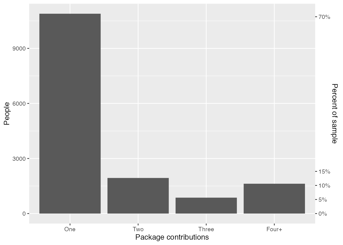
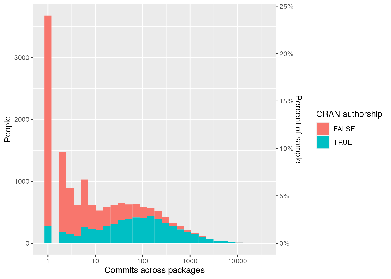
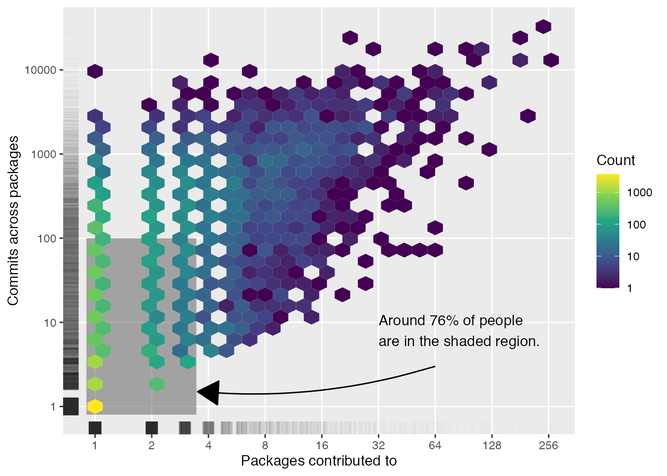
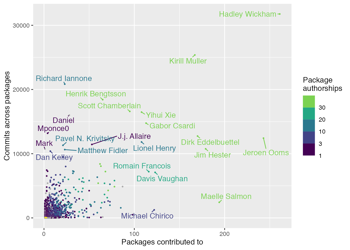
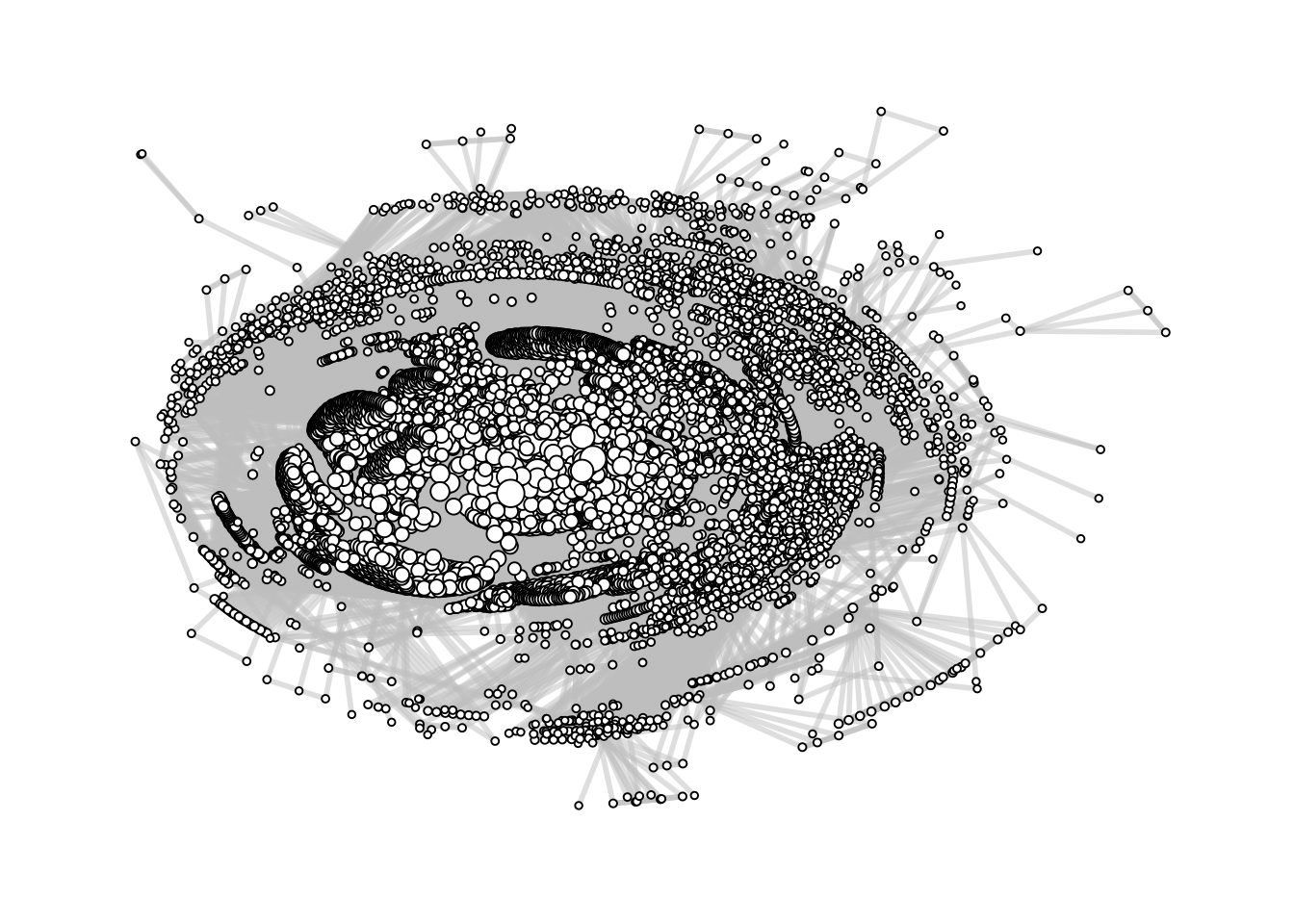
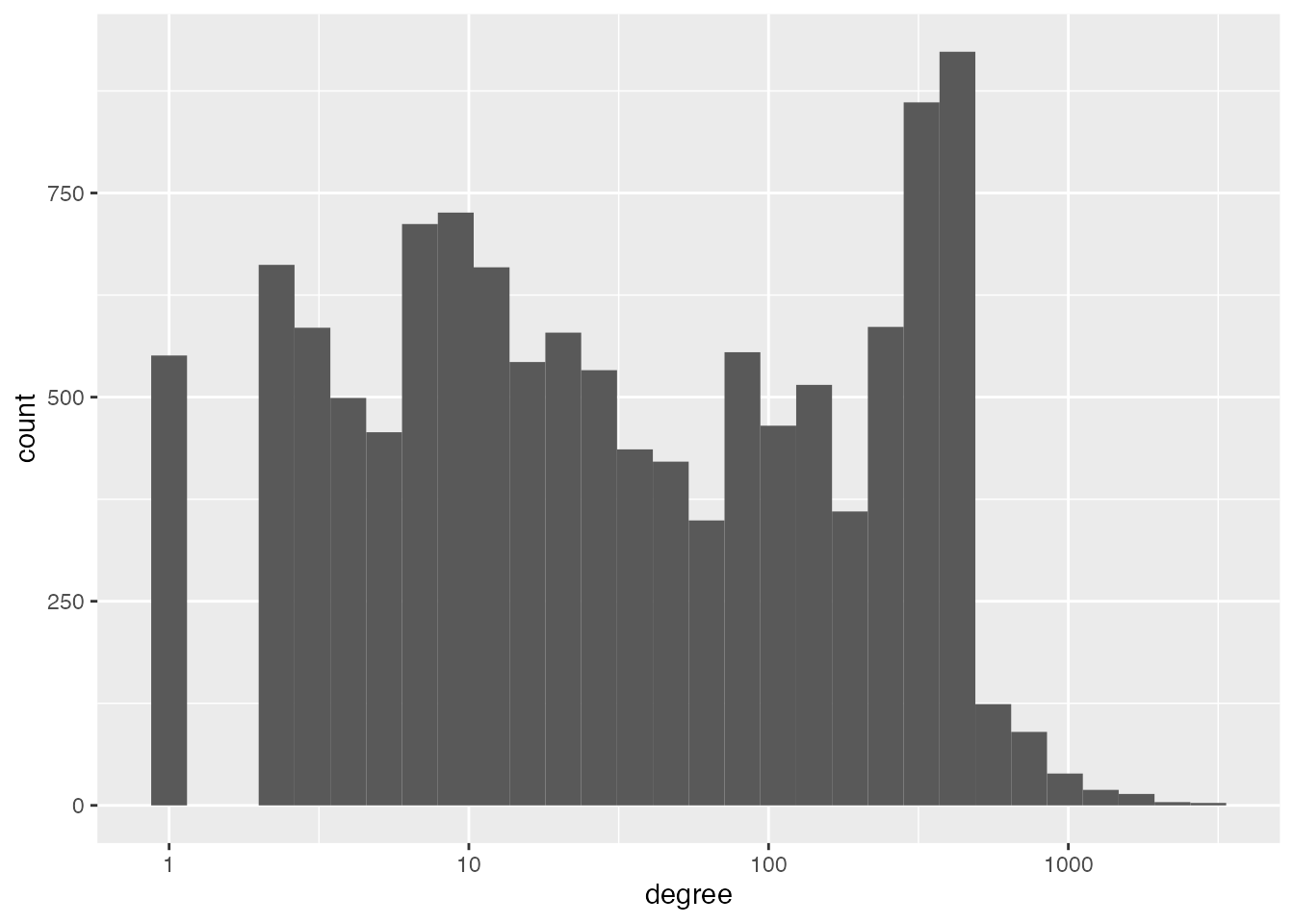
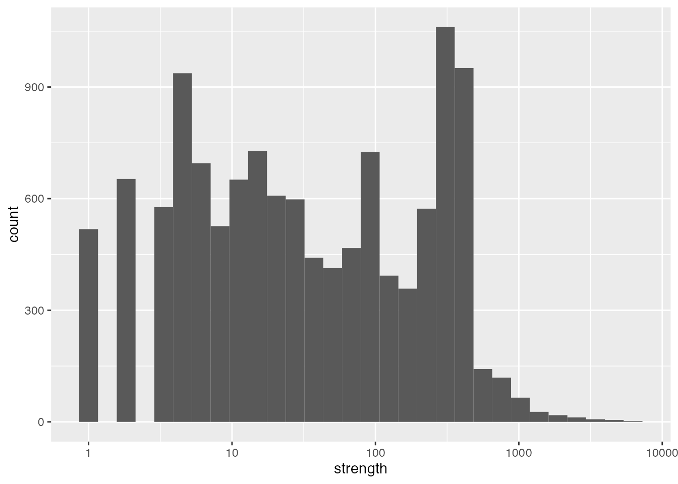
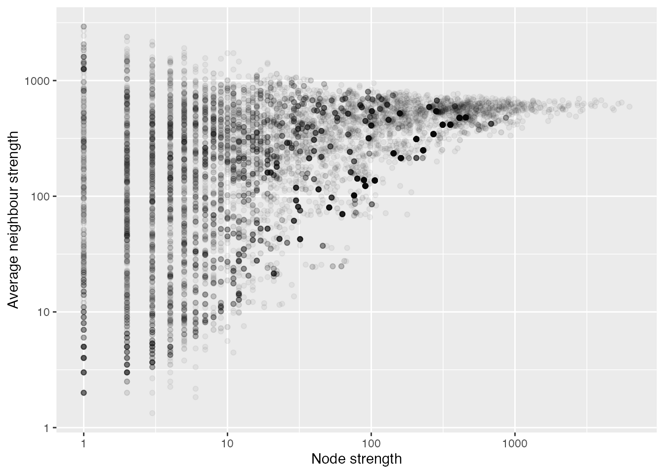
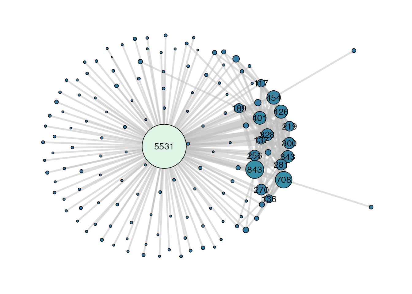
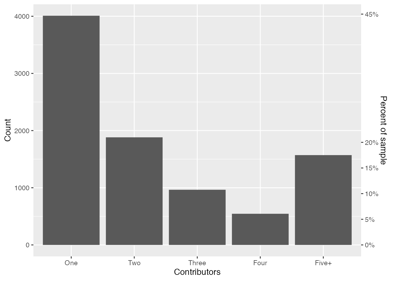
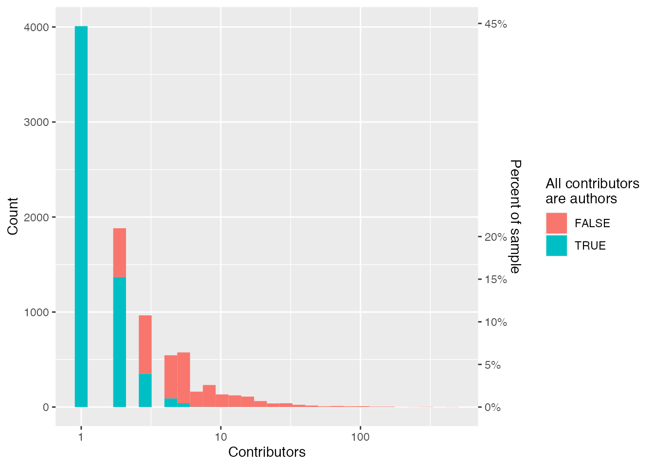
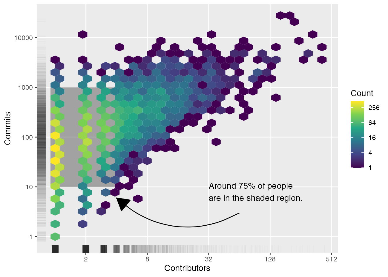
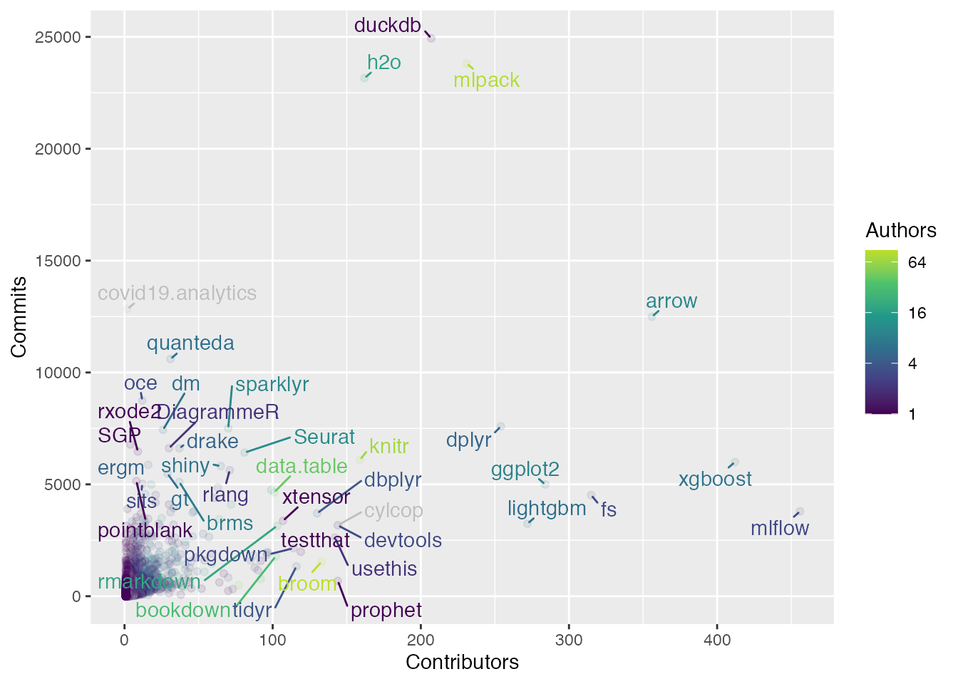
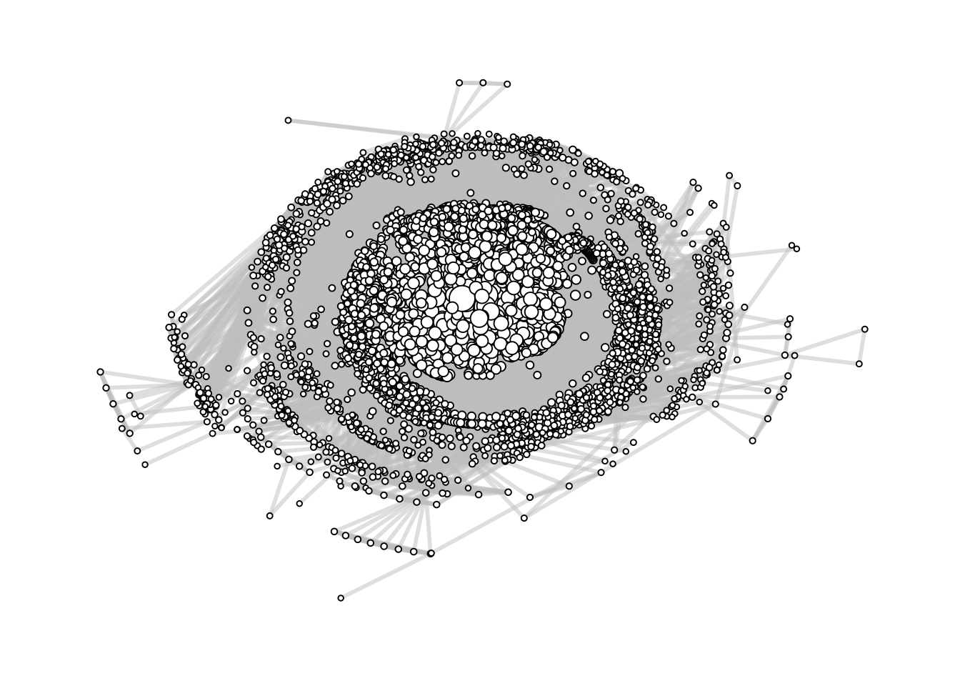
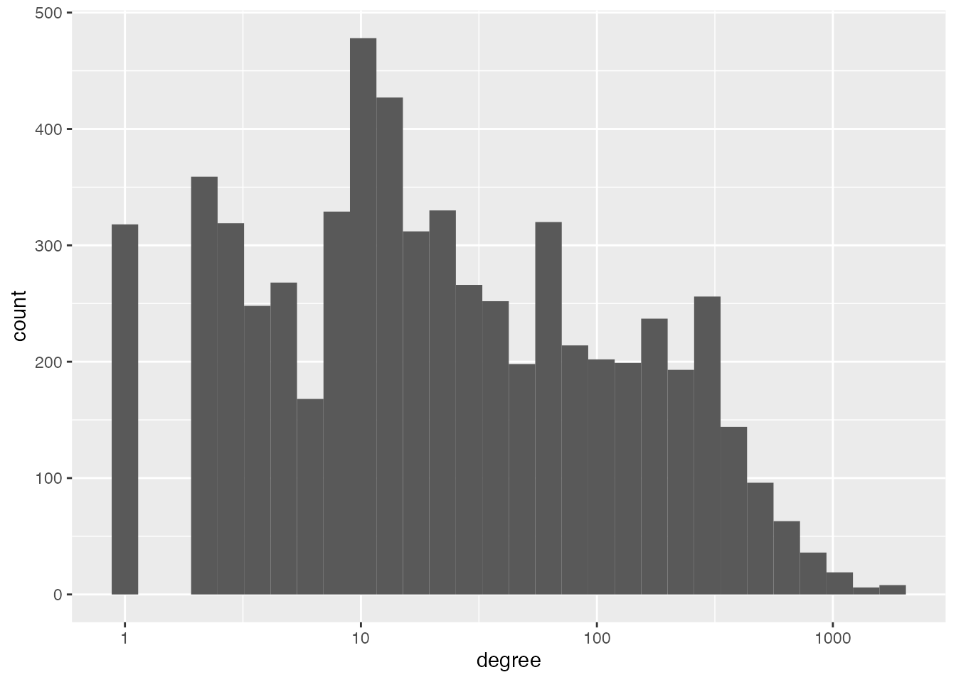
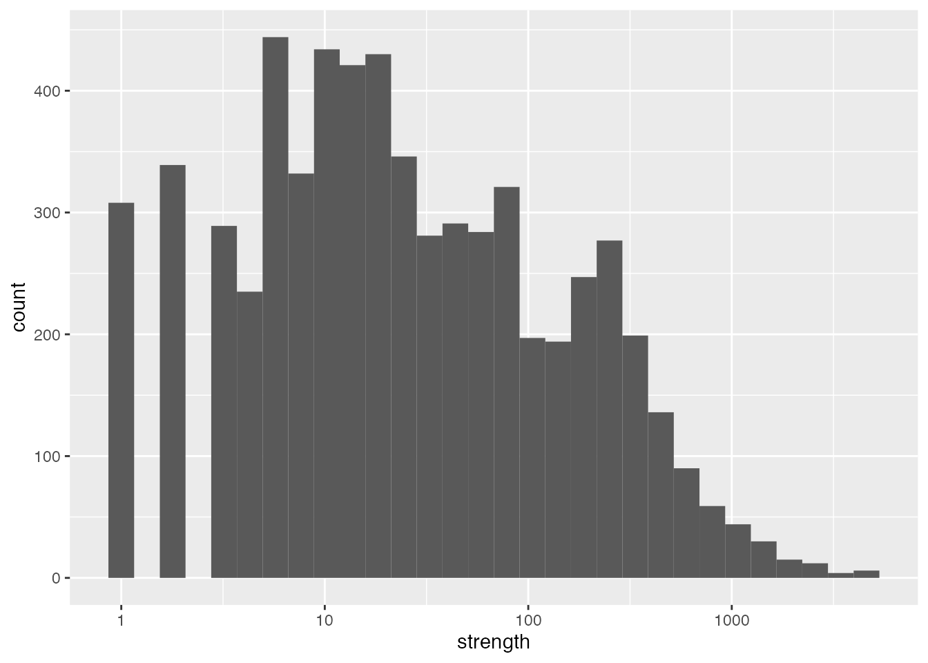
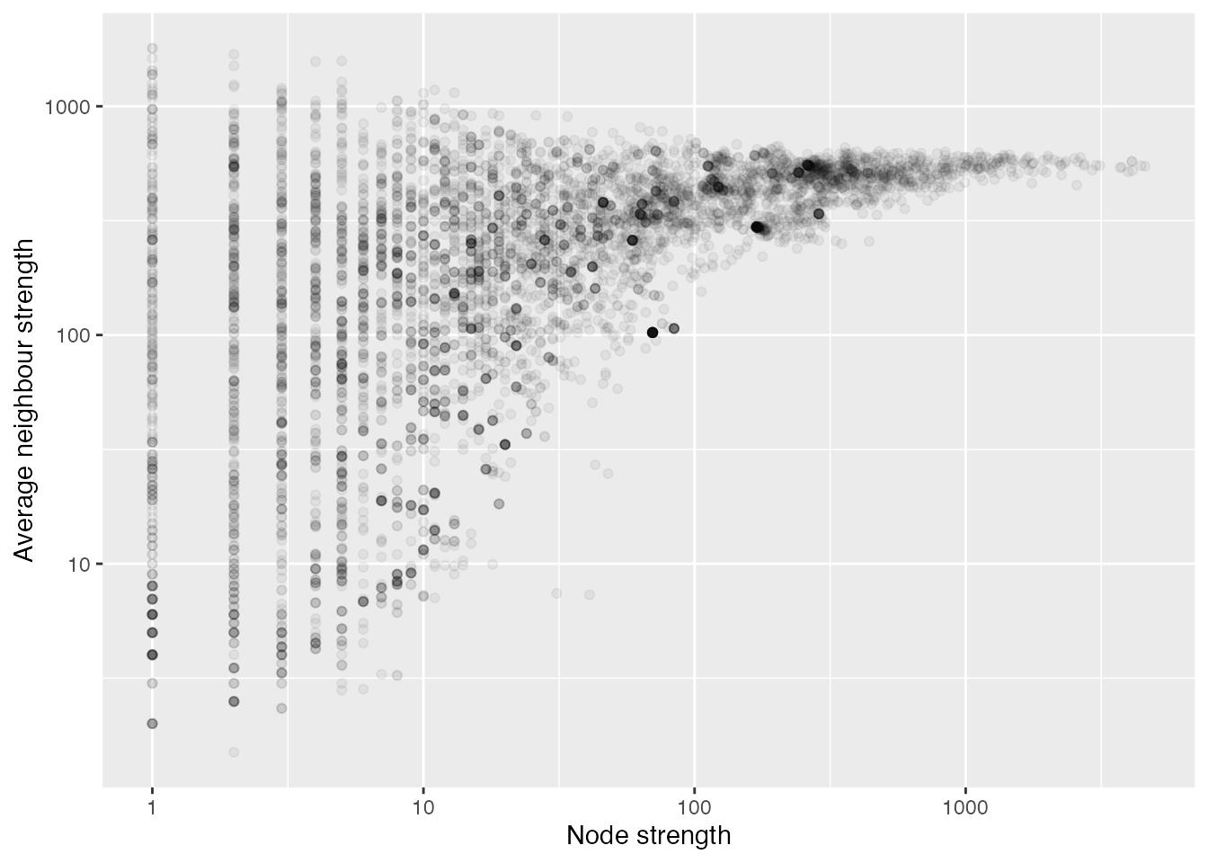
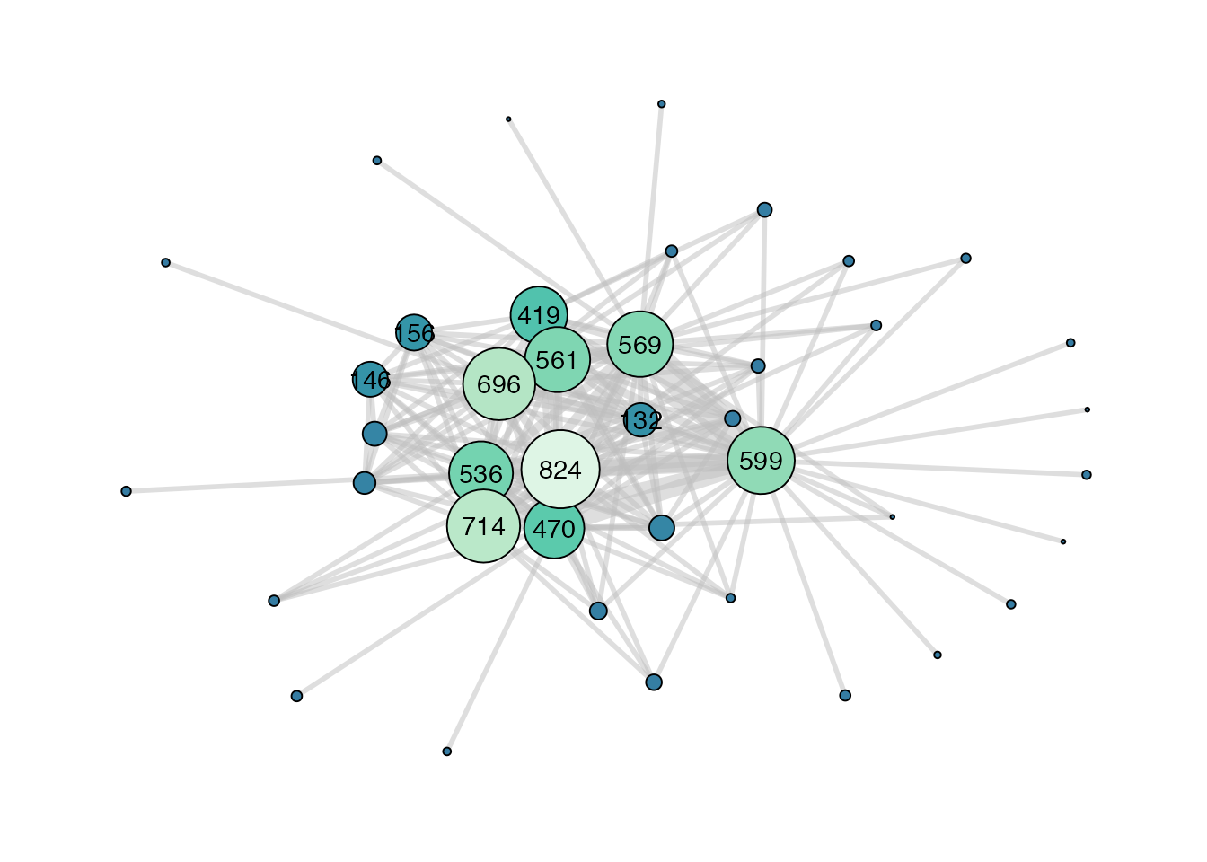
Comments